Behavior Research Methods, Instruments, & Computers 2003, 35 (2), 285-293
Scaling techniques for modeling directional knowledge DAVID WALLER University of California, Santa Barbara, California and DANIEL B. M. HAUN University of South Carolina, Columbia, South Carolina A common way for researchers to model or graphically portray spatial knowledge of a large environment is by applying multidimensional scaling (MDS) to a set of pairwise distance estimations. We introduce two MDS-like techniques that incorporate people’s knowledge of directions instead of (or in addition to) their knowledge of distances. Maps of a familiar environment derived from these procedures were more accurate and were rated by participants as being more accurate than those derived from nonmetric MDS. By incorporating people’s relatively accurate knowledge of directions, these methods offer spatial cognition researchers and behavioral geographers a sharper analytical tool than MDS for studying cognitive maps.
As people gain experience with their surroundings, they develop a mental representation of the environment that allows them to make inferences about spatial relationships that they have never directly experienced. For example, after traveling, on different occasions, between two locations on campus, a student may deduce that there is a short-cut between them that he or she can take to save time. The knowledge that emerges as a result of transforming groundlevel egocentric perceptual experiences into a flexible representation of global relationships in an environment is often referred to as a cognitive map (Downs & Stea, 1977; Gallistel, 1990; Golledge, 1999; O’Keefe & Nadel, 1978; see also Kuipers, 1982). Much of the current interest in spatial cognition and environmental psychology concerns the nature of cognitive maps. As a result, analytical tools that allow investigators to model, describe, or illustrate the nature of cognitive maps are extremely valuable to the field. One of the most widely used quantitative methods for modeling cognitive maps is multidimensional scaling (MDS), which, conceptually, transforms information that is available from ground-level experience into more global knowledge (Kruskal & Wish, 1978; Shepard, 1980). When used to model spatial knowledge, MDS algorithms have traditionally been used to transform one-dimensional information about the distances between places into a higher dimensional metric representation—a map—of the enviThis research was conducted with support from the U.S. National Science Foundation, Grant 9873432. We thank Reginald Golledge, Yvonne Lippa, Jack Loomis, Dan Montello, and Waldo Tobler for helpful comments on earlier drafts. Correspondence concerning this article should be addressed to D. Waller, Department of Psychology, Miami University, Oxford, OH 45056-1601 (e-mail:
[email protected]).
ronment. (Although a class of models [such as principal components analyses] that do not require distance information can be considered as variants of MDS, these models have generally not been applied to environmental knowledge and are not considered further in this paper.) For example, a person’s estimates of the distances between various cities in the United States can be submitted to an MDS algorithm to generate a map that maximally fits the estimates, creating a configuration of cities much like the actual topographic layout. Nonmetric versions of MDS can also recover a similarly accurate topographic layout based only on the ordinal properties of people’s distance estimates. Although it is generally considered to be quite useful in describing or portraying mental representations of space, MDS has one major drawback: It relies exclusively on estimations of distances between locations. For most people, estimating distances is not a well-practiced task. As a result, the accuracy of distance estimations can exhibit high variability between people (Da Silva, Ruiz, & Marques, 1987; Fine & Kobrick, 1983; Sharrack & Hughes, 1997). In our own experience, we have found that when experimental participants are told that they will be asked to point and estimate distances to and from various locations, many try to warn us about how poorly they expect to do with their distance estimations. Yet very few people balk similarly at making directional estimations by pointing. Because people appear to have more confidence in judging directions than distances, we were interested in examining approaches to MDS that incorporate people’s directional knowledge. In this paper, we examine two alternative approaches to MDS, each of which uses information about directional relationships in converting a set of onedimensional judgments into a two-dimensional map. After
285
Copyright 2003 Psychonomic Society, Inc.
286
WALLER AND HAUN
describing these two scaling techniques, we will report an experiment that illustrates their potential utility. We will show that both of these algorithms can produce maps that are more likely than MDS-derived maps to be selected as representing the actual environment. From these results, we will argue that scaling algorithms that incorporate people’s directional knowledge offer researchers a sharper analytical tool than traditional MDS does in modeling cognitive maps. We begin, though, with a brief examination of the role of MDS in spatial cognition research. MDS in Spatial Cognition Research Since its introduction (Torgerson, 1952) and early development (Kruskal, 1964a, 1964b; Shepard, 1962a, 1962b), MDS has been a popular technique for modeling proximity data that arise in many branches of psychology (see, e.g., Carroll & Arabie, 1980; Shepard, Romney, & Nerlove, 1972). Although some of these applications of MDS have been criticized for portraying inherently nonmetric data in a metric space (Tversky, 1977; Tversky & Gati, 1982), the use of MDS in the domain of spatial cognition is probably one of the more credible applications. This is because the space that is ultimately represented by the individual (i.e., the actual environment) has a known structure that closely approaches that of a metric space. Although people’s distance estimates do not always obey the axioms that are necessary for a metric space (Sadalla, Burroughs, & Staplin, 1980), most investigators agree that MDS is a valuable tool for interpreting and visualizing aspects of the latent structure inherent in a set of distance estimations. As a result, MDS has been used extensively in the field of spatial cognition (Allen, Siegel, & Rosinski, 1978; Brown & Broadway, 1981; Foley & Cohen, 1984; Golledge, Rayner, & Rivizzigno, 1982; Haber, Haber, Levin, & Hollyfield, 1993; Howard & Kerst, 1981; Kitchin, 1996; Kosslyn, Pick, & Fariello, 1974; Lockman, Rieser, & Pick, 1981; Regian & Yadrick, 1994). Most investigators that have used MDS to model internal spatial representations have preferred not to make metric assumptions about participants’ data and have used the nonmetric version of MDS developed by Shepard (1962a, 1962b) and Kruskal (1964a, 1964b). It is important to recognize that there are two ways in which a scaling technique such as MDS can be said to provide valid or accurate results. First, maps generated by the technique can accurately depict people’s mental representation of an environment. Second, such maps can accurately depict the environment itself. We refer to the latter type of accuracy as veridicality and note that, in general, the veridicality of a map is much easier to assess than is its psychological accuracy. Several studies have examined the veridicality of MDS-derived maps relative to those derived from other techniques (Baird, Merrill, & Tannenbaum, 1979; Buttenfield, 1986; MacKay, 1976; Magaña, Evans, & Romney, 1981; Richardson, 1981). Most— although not all—of these studies have concluded that the knowledge represented in sketch maps is either more veridical or more precise than knowledge represented with MDS. This result is not unequivocal, though. For ex-
ample, Buttenfield (1986) compared distortions in MDS configurations with those for sketch maps and concluded that MDS-generated maps were more veridical (although also more variable) depictions of the environment than were participants’ sketch maps. Findings about the veridicality of maps generated by MDS can inform investigators about the degree to which people’s knowledge of environmental relationships corresponds to reality. As such, these studies can be helpful in predicting or understanding biases and errors in performance on spatial tasks. Determining whether a derived map accurately reflects a person’s mental representation of an environment is a much more challenging issue, and one that few studies using MDS have addressed (but see Baird et al., 1979; MacKay, 1976). In the present research, we approached the issue of psychological accuracy in two ways. First, we asked participants to construct an unconstrained map representing the configuration of a set of familiar landmarks. We then used this explicitly constructed map as a representation of their cognitive map. Such a technique is relatively common in the spatial cognition literature (see, e.g., Baird et al., 1979; Huertas & Ochaita, 1992; Sherman, Croxton, & Giovanatto, 1979; Waller, 2000; Walsh, Krauss, & Regnier, 1981). Comparisons between participants’ explicitly constructed maps and those derived from MDS and other scaling techniques can inform us about the relative ability of these techniques to represent peoples’ cognitive maps. Second, we asked participants to rate the veridicality of maps derived from MDS, as well as from other methods. Making such ratings requires participants to compare a stimulus map with a spatial representation held in memory and, thus, may provide some insight into the nature of people’s cognitive representation of an environment. Such an approach was taken by MacKay (1976), who examined people’s knowledge of the relative locations of cities in the United States. In addition to showing that hand-drawn maps were more veridical than those derived from MDS, MacKay found that hand-drawn maps were more likely to be rated as representing the true configuration of cities than were maps generated from nonmetric MDS. MacKay (1976) explained these results by suggesting that graphic methods, such as sketch maps, may offer investigators keener insight into the nature of cognitive maps, because they allow expression of both distance and directional knowledge. The degree to which MacKay’s results apply to spatial knowledge gained as a result of navigation in the environment is not clear. Certainly, though, his suggestion that the utility of MDS is limited by its failure to account for angular relationships applies to the use of MDS in modeling spatial data at all scales. In the next section, we will discuss our development of tools that allow us to examine more closely MacKay’s intuition that MDS, by not accounting for directional relationships, does not adequately represent the spatial knowledge contained in people’s cognitive maps. Including Directional Information in MDS One approach to scaling directional information was suggested in an algorithm introduced by Gordon, Jupp, and
MODELING DIRECTIONAL KNOWLEDGE Byrne (1989). Their technique is similar to MDS, inasmuch as it constructs a two-dimensional map that maximally fits a set of pairwise estimates. However, unlike MDS, this method takes pairwise estimates of directions (i.e., the estimated degrees clockwise from north from one location to another) as input. To illustrate their algorithm, Gordon et al. used distance and bearing estimations from one person to create two different maps—one based on their technique and the other based on a distance scaling procedure similar to nonmetric MDS. The resultant maps for this person appeared to be quite different from each other, and the map based on angular information more closely matched the actual configuration of locations. A more experimental approach was taken by Wender, WagenerWender, and Rothkegel (1997), who adopted Gordon et al.’s technique and showed that when data are averaged across many participants, Gordon et al.’s algorithm—as well as nonmetric MDS—produces veridical representations of a recently studied map. Wender et al.’s data suggested that MDS produces maps that are in fact more veridical than those produced by Gordon et al.’s technique; however, this difference was neither large nor significant. Several aspects of Wender et al.’s experiment may limit its applicability to the questions to which the present paper is addressed. For example, Wender et al. examined memory for recently studied maps. In the present study, we focused on modeling environmental knowledge gained as a result of extensive navigation within a known environment. Like the algorithm suggested by Gordon et al. (1989), our first scaling procedure (which we call ANGSCAL) constructs a best-fitting map from a set of pairwise bearing estimates. Intuitively, ANGSCAL starts with a configuration of points and rearranges their locations until the difference between the interpoint directions in the configuration and the estimated interpoint directions is as small as possible. More formally, given a set of interpoint bearings qij (measured in degrees) that represent estimated directions from the i 5 1. . . n to the j 5 1. . . n (i ¹ j ) locations, we create an n 3 2 matrix X, representing a two-dimensional configuration of n points. Let the interpoint bearings of X be denoted qˆij, such that æ xi 2 - x j 2 ö qˆij = (90 × K ) - tan -1 ç ÷, è xi1 - x j1 ø
where K 5 1 when xj1 . xi1 and K 5 3 when xj1 , xi1. The method then finds the configuration X that minimizes Stress A =
(
)
1 × å q ij @ qˆij , n( n - 1) i ¹ j
where the operator @ represents an unsigned bearing difference bounded by 180º (i.e., q 1 @ q 2 5 min{|q 1 2 q 2|,|q12(q 2 1 360)|,|(q 1 1 360)2q2|}). In our applications, StressA is minimized using a commercially available optimization procedure based on a quasi-Newton minimization algorithm (Broyden, 1970; Fletcher, 1970; Goldfarb, 1970; Shanno, 1970). ANGSCAL is conceptually very similar to the procedure proposed by Gordon et al. (1989; see also Tobler,
287
1996); however, instead of minimizing a measure of stress based on the cosine of the differences between the observed and the derived bearings, we optimize their mean absolute deviation. We note that our stress formula and Gordon et al.’s stress formula are monotonically related and correlate extremely highly (r 5 .993) with each other. However, we feel our criterion is a more natural measure of angular difference and is more sensitive to smaller bearing differences. If one weakness of MDS is that it uses only distance information in deriving configural representations of spatial knowledge, ANGSCAL clearly has the converse weakness: It uses only directional information. Clearly, people’s mental representations of space allow successful performance on tasks that require judgments of either distances or directions. It thus seems likely these mental representations code both types of information (see, e.g., Cheng, 1998, or Chieffi & Allport, 1997). Thus, a scaling procedure that incorporates both kinds of information may yield more valid representations of cognitive maps. Our second scaling algorithm (called DANSCAL, for distance and angular scaling) works similarly to the one described above; however, it incorporates both distance and bearing information into the minimization criterion. Given a set of bearing estimates (qij ) and a set of distance estimates (dij ) that represent estimated distances from the i 5 1. . . n to the j 5 1. . . n (i ¹ j) locations, the DANSCAL algorithm creates an n 3 2 matrix X representing a two-dimensional configuration of n points. If the interpoint bearings of X are denoted qˆij (defined as in ANGSCAL) and its interpoint distances are denoted dˆij, such that dˆij =
( xi1 - xi1) + ( xi2 - xi2 ) 2
2
,
we find the configuration X that minimizes Stress B =
å d ij2 + dˆij2 - 2 × cos(q ij @
i¹ j
)
qˆij × d ij × dˆij .
As before, the @ operation signifies an unsigned bearing difference.1 In our application of this technique, StressB is minimized using the same optimization algorithm as that used for StressA. It is instructive to note that this formula combines distance and directional information by way of the law of cosines. If the distance (d ) and bearing (q ) information for any pair of locations are considered as twodimensional vectors with magnitude d and direction q, this formula works by computing the distances between the endpoints of all corresponding pairs of these vectors (see Figure 1). This technique is similar in spirit to a scaling algorithm proposed by Everittt and Gower (1981). Like DANSCAL, Everitt and Gower’s technique incorporates bearing and distance information into a to-be-minimized stress formula. However, Everitt and Gower’s stress criterion lacked a straightforward geometric interpretation and, to our knowledge, has never been applied to data involving spatial cognition. We were interested in determining the relative veridicality, precision, and preferences for maps produced by nonmetric MDS, ANGSCAL, and DANSCAL. University
288
WALLER AND HAUN computer rendered these scenes using a Pentium III chipset and an NVIDIA GeForce2 MX graphics card, updating the graphics and display at 72 Hz. Randomization and presentation of the stimuli, as well as the collection of pointing and distance estimations, were controlled through a scripting facility in the Python programming language, supplemented with a utility module written by Andrew Beall specifically for virtual environment applications. More information about the validity of this assessment method is available from Waller, Beall, and Loomis (2002).
Figure 1. The geometric interpretation of the formula for DANSCAL. The distance ( d ) and direction (u ) between two locations that are judged by the participant are represented as the solid vector. The distance (d ˆ ) and direction (u ˆ ) in the derived configuration are represented as a dashed vector. The minimization criterion for this pair of vectors is the distance between their endpoints—the dotted line.
undergraduates were asked to make distance and direction judgments about familiar campus locations and were also asked to construct a map of the campus environment. Each participant’s pointing and distance data were then submitted to the three scaling algorithms, producing three maps of campus. The participants rated the accuracy of these maps, as well as the map they constructed and the actual map of campus. METHOD Participants Twenty-eight students (14 men and 14 women) from the University of California, Santa Barbara, participated in the experiment. The participants received either extra credit in their introductory psychology class (n 5 14) or a payment of $10 (n 5 14). All the participants reported being familiar with the campus. Environment and Materials The environment that was tested consisted of six locations on the campus of the University of California in Santa Barbara. Each location was near a prominent campus landmark (the Library, the Student Center, the Recreation Center, two campus entrances, and a local restaurant), and none of the locations was visible from the others. The positions of these locations (and hence, their relative distances and directions) were determined with a Garmin GPS 12XL global positioning system, accurate to at least 15 m. The participants were tested in the laboratory, in computergenerated simulations of each of the six locations. These simulations were created from 360º panoramic photographs of each location that were applied to the inside surface of a computer-modeled cylinder. The user’s viewpoint was placed in the center of the cylinder. The participants viewed these panoramas using a V8 head-mounted display (HMD) from Virtual Research. The display provided 640 3 480 pixel resolution with a 38º horizontal field of view. Mounted on the HMD was an inertially based orientation tracker (Intersense Model IS-300). The tracker was used to update the orientation of the visual image as the participant moved his or her head, as well as to record the facing directions in the pointing task described below. The
Procedure The participants were run individually through the following four phases of the experiment: (1) assessment of the participant’s familiarity with the to-be-tested locations, (2) pointing and distance estimations, (3) map construction, and (4) rating of the maps produced by different algorithms. Assessment of the participants’ familiarity with the locations began by showing them the six panoramas in a fixed order in the HMD. When the participant identified each location (which never failed to happen), the experimenter gave it a short memorable name that was used as a label for the rest of the experiment. The participants then were asked to point and estimate distances to and from all pairs of these locations. For both distance and direction estimates, the simulated testing location was perceptually available in the HMD to the participants. A distance judgment always followed each direction estimation. Five of these direction/ distance pairs were given in six blocks, one for each location, resulting in 30 direction and distance estimates. For direction estimations, the participants were shown each appropriate testing location in the HMD and then were asked to face each of the other locations (targets). While direction estimates were provided, a red arrow in the center of the screen was overlaid on the depicted testing location to assist the participants with lining up their estimated direction. After pointing to each target, the participants were asked to estimate verbally the straight (Euclidean) distance to the target. The participants were instructed that they could use any unit of distance that they wanted and that it was more important for their distance estimates to maintain relative (rather than absolute) accuracy. As a reference, the participants were reminded that meters and yards were of similar length and that there were 100 yards in a football field. The presentation order of the six simulated locations, as well as each of the five pointing locations for each one, was randomized for each participant. The participants’ verbal distance estimates (entered by the experimenter) and their motoric bearing estimates (i.e., their facing directions) were automatically written to an external computer file for later analysis. Next, the participants were asked to construct a map of the environment from memory by placing small cardboard pieces representing the six locations on a blank sheet of grid paper. The x- and y- coordinates of the participants’ map placements were recorded for later analysis. The participants then waited for about 5 min while the mapgenerating routine ran. This routine created a set of nine maps, each consisting of six labeled points that represented a different configuration of the six campus landmarks. It then printed each one on a different sheet of paper. The configuration on each of these maps was rigidly rotated and scaled with (an affine version of) bidimensional regression (Tobler, 1994; see also Kitchin, 1996) to maximally fit the orientation of the participant’s constructed map. Bidimensional regression is a statistical technique that determines the amounts by which a two-dimensional configuration must be translated, rotated, and scaled so that it can be superimposed on another configuration with as little difference as possible. This procedure yields estimates of these transformations, as well as a measure of how similarly shaped the two configurations are. This bidimensional correlation r (BDr) is very analogous to, and can be interpreted as, a typical bivariate correlation coefficient (Gatrell, 1983; Nakaya, 1997; Tobler, 1976; Wakabayashi, 1994). The first three maps
MODELING DIRECTIONAL KNOWLEDGE
289
other scaling algorithm not reported in this paper.) These five maps were presented in a different random order for each participant. The computer checked the MDS configuration to verify that it was not a reflected version of the participant’s map. If it was, the MDS map was reflected before it was fit to the participant’s map placement data. The ninth map shown to the participants was the actual map of the campus locations. The participants were instructed to study each map separately and to rate each one on a scale from 1 to 7, where 1 meant that it was completely distorted and 7 meant that it was perfectly accurate . The participants were not told that the first three maps were serving as anchors for their rating scale, nor were they told that any of the maps were their own or the actual map. The participants’ ratings for the MDS, ANGSCAL, DANSCAL, map placement, and actual maps were recorded for later analysis.
RESULTS
Figure 2. Mean ranking (and standard errors) for the ratings of maps produced by three scaling techniques, the map placements, and the actual configuration.
shown to the participants were the same for all the participants and were used to illustrate implicitly the possible range of distortions that subsequent maps could be expected to contain. The first map was a fairly accurate map of the campus (BDr with the actual configuration 5 .96). This was followed by one that was more distorted (BDr 5 .82), followed by one that was very distorted (BDr 5 .29). The next five maps contained those generated from nonmetric MDS,2 ANGSCAL, and DANSCAL, as well as the map portraying their map placements. (The fifth map in this set was derived from an-
To verify that the ANGSCAL and DANSCAL algorithms had converged on global minima, for both procedures, each participant’s data were later rerun from another set of starting values and were allowed to converge again to a solution. These results were then compared with those that had been shown to the participant. Data from 8 participants were eliminated because the ANGSCAL map that they were shown either had not converged or had converged on what was later determined to be a local minimum. For these participants, when ANGSCAL was allowed to converge on a global minimum, it produced a map that was perceptibly different (BDr , .99) from the one they were shown. For the remaining 20 participants (10 men and 10 women), the ANGSCAL and DANSCAL procedures run during the experiment either were later
A
F
E
C D B
N 0
50
100 m
Map placement MDS DANSCAL ANGSCAL Actual location
Figure 3. Five of the configurations generated for and rated by 1 participant. For this figure, the five configurations were combined using Procrustes superimposition (described in the text). Corresponding locations on each map were then connected to the actual location. The participants rated the accuracy of each map separately.
290
WALLER AND HAUN
Table 1 Interpoint Distance Estimates (From Row to Column) Given by the Participant Whose Data are Illustrated in Figure 3 A A B C D E F
250 300 160 175 75
B
C
D
E
F
400
400 75
200 180 400
120 225 160 320
90 200 410 110 175
90 240 200 300
300 80 400
420 100
275
judged to have converged on a global minimum or else had converged to a solution that resulted in a map that was extremely similar (BDr . .99) to that implied by the global minimum found later. The remaining analyses were conducted only on this set of 20 participants. For each participant, the ratings given for the MDS, ANGSCAL, DANSCAL, map placement, and actual configurations were ranked (assigning mean ranks to ties). Mean ranks for the ratings of the different configurations are shown in Figure 2. In general, MDS was rated as being the most distorted configuration (mean rank 5 2.20, SD 5 1.22), and the participants’ map placements were rated as being the most accurate (mean rank 5 4.45, SD 5 1.71). Maps produced by ANGSCAL (mean rank 5 4.20, SD 5 1.28) were rated as being slightly less accurate than those produced in the map placement task. The actual configuration of locations (mean rank 5 3.55, SD 5 1.66) and configurations based on DANSCAL (mean rank 5 3.20, SD 5 1.40) were rated similarly—both slightly lower than ANGSCAL. These five rated maps from 1 representative participant are shown in Figure 3. This participant’s distance and bearing estimates, from which these maps were derived, are presented in Tables 1 and 2. Differences between the rankings of the ratings for these configurations were tested in a 2 (gender) 3 5 (configuration) analysis of variance (ANOVA), with the latter factor represented with repeated measures.3 This ANOVA revealed a significant omnibus effect of configuration [F(4,15) 5 7.91, p 5 .001]. Planned pairwise contrasts revealed that most of this effect was due to the relatively low ranking of MDS. MDS was ranked significantly lower than DANSCAL [t(18) 5 2.11, p 5 .049], ANGSCAL [t(18) 5 5.88, p , .001], map placements [t(18) 5 4.26, p , .001], and the actual configuration [t(18) 5 2.77, p 5 .013]. Pairwise contrasts between the mean rankings for the non-MDS configurations were not significant. Gender did not significantly affect the participants’ ratings [F(1,18) 5 0.19, p 5 .667], nor did it interact with the effect of configuration [F(4,15) 5 0.28, p 5 .886]. To examine relationships among the five maps illustrated in Figure 3, we computed for each participant a set of bidimensional correlations that represented the similarity between all possible pairs of the five configurations. Mean bidimensional correlations between the configurations derived from the different methods appear in Table 3. In general, the maps derived from all three scaling procedures were more similar to the actual configuration than
they were to people’s map placements. Indeed, the maps derived from ANGSCAL were extremely similar to the actual layout (mean BDr 5 .96). This reflects the fact that, on average, the participants’ bearing estimations were quite accurate. Mean signed bearing error ranged from –8.97º to 4.97º across all participants and averaged –0.76º (SD 5 3.71º). Maps derived from MDS were less similar to the actual layout (mean BDr 5 .83) than those derived from ANGSCAL or DANSCAL. Relationships among the various configurations are depicted in Figure 4. To create Figure 4, the x- and ycoordinates of the derived configuration for each method were averaged with Procustes superimposition(Dryden & Mardia, 1998). Procrustes superimposition has the effect of translating, rotating, and scaling (dilating) each participant’s configuration optimally to derive an average configuration across all participants. Each participant’s data, relative to this average configuration, form a point cloud around each location. Standard ellipses summarize these point clouds by enclosing approximately 40% of the observations (see Batschelet, 1981). Most notable in Figure 4 are the relatively small ellipses associated with ANGSCAL. In addition to providing the most veridical configurations (see Table 3), ANGSCAL also appears to have less variability than the other methods. DISCUSSIO N In this experiment, the participants rated the veridicality of maps derived from three different methods of scaling pairwise estimations of directions and distances. The participants’ ratings were directly related to the degree to which the scaling procedure incorporated directional information. Maps that were derived exclusively from distance information (using nonmetric MDS) were consistently rated as being more distorted than those derived exclusively from directional information (using ANGSCAL). The technique incorporating both distance and direction information (DANSCAL) was rated between these two extremes. Maps derived from ANGSCAL were rated as being nearly as accurate as maps that the participants had recently constructed. Part of this is probably because ANGSCAL maps were, in fact, extremely veridical depictions of the environment—much more accurate than those derived from other techniques. We will discuss the
Table 2 Interpoint Bearing Estimates (Degrees Clockwise From North From Row to Column) Given by the Participant Whose Data are Illustrated in Figure 3 A A B C D E F
341 307 46 261 69
B
C
D
E
F
164
135 68
200 273 252
90 59 55 62
247 308 279 12 279
214 85 220 93
75 225 84
253 189
72
MODELING DIRECTIONAL KNOWLEDGE
291
Table 3 Mean Bidiminesional Correlations Between Configurations Produced by Three Scaling Methods, the Map Placement Task, and the Actual Configuration DANSCAL ANGSCAL Placement Actual
MDS
DANSCAL
ANGSCAL
Placement
.84 .83 .81 .83
.92 .87 .90
.90 .96
.89
psychological implications of these findings below, after a brief discussion of several caveats to our conclusions. One possible reason that the inclusion of directional information yielded maps that were (and were perceived to be) more veridical than those using distance information involves the method we used to assess directional knowledge. In the present study, we measured the participants’ directional knowledge while they were immersed in a photo-realistic computer simulation of each location. We have recently shown in another experiment that this assessment technique produces less measurement error than do those based on more traditional assessment techniques, such as paper-and-pencil methods (Waller et al., 2002). By simulating the testing environment, we relieved the participants of the need to imagine these locations and enabled them to use landmarks and local directional cues (such as streets and walkways) to inform their answers. As a result, the participants’ answers were probably very close to those they would have supplied if they had been tested at the actual locations and, in this sense, were probably more valid indicators of their directional knowledge
N 0
50
100 m
(see Waller et al., 2002). On the other hand, the degree to which our assessment method aided the participants in making distance judgments seems less apparent. Unlike the motoric responses we obtained indicating directions, distance estimations were produced verbally and were thus likely to have been influenced by higher level cognitive strategies or heuristics. It is possible that other methods of eliciting distance estimations (see Montello, 1991) would have produced results that were more favorable to MDS. This is clearly a question for further investigation. Another factor that may limit the scope of our conclusions involves the relatively small stimulus set size in the present experiment. By testing only six locations, we may have adversely impacted the effectiveness of MDS in representing the environment adequately. It is generally thought that two-dimensional MDS solutions should be derived from stimulus sets with eight or more items in order to avoid spurious solutions (Kruskal & Wish, 1978; Schiffman, Reynolds, & Young, 1981). Importantly, however, in the present case, because we did not assume that distance estimates would be symmetrical, the participants
Map placement MDS DANSCAL ANGSCAL Actual location
Figure 4. Standard ellipses (see Batschelet, 1981) for estimated locations derived from different map-making techniques. For each method, the x- and y-coordinates of the derived configuration were averaged with Procrustes superimposition (Dryden & Mardia, 1998).
292
WALLER AND HAUN
supplied twice as many pairwise estimates as are used in most studies with MDS. Thus, our MDS procedure had relatively high degrees of freedom (30) from which to compute its 12 coordinates. It is generally believed that the use of MDS is warranted when the ratio of degrees of freedom to estimated parameters exceeds two (Kruskal & Wish, 1978). In any event, it is important to note that in the present experiment, ANGSCAL and DANSCAL were both based on the same relatively small stimulus set size, yet both reached more accurate and more preferred solutions than did MDS. Our results suggest, then, that from a practical perspective, the reliance of MDS on larger stimulus set sizes is perhaps another of its weaknesses. Of course, it is important, from a theoretical perspective, to understand the degree to which MDS models based solely on distance information are able to represent people’s knowledge of environmental relationships. This, too, remains an issue for more research. In our study, scaling methods based on directional knowledge were consistently rated as yielding more veridical maps than were those based on distance information. Although it would be naive to conclude from this finding that angular information is more prominently represented in people’s mental representation of an environment, our findings clearly imply that people’s knowledge of directions in a familiar environment contains information that corresponds more closely to performance on tasks that require the adoption of a bird’s-eye perspective than does knowledge of distances. To the extent that either map construction tasks or veridicality ratings of spatial configurations measure cognitive maps, ANGSCAL and DANSCAL appear to offer more valid measures of internal spatial representations. Another important finding concerns the absolute and relative accuracy of maps produced by the different scaling methods. Averaged over all of their estimations, the directional knowledge of our participants was quite accurate and showed no evidence for systematic biases. This relatively error-free directional knowledge resulted in ANGSCAL maps that were exceptionally accurate depictions of the environment—more accurate than the participants’ map placements. The difference in veridicality between maps that were constructed and those that were derived from ANGSCAL suggests that the two configurations either were based on different internal representations or resulted from different task-related mental processes. In future research, we hope to distinguish empirically between these two alternatives. By employing scaling techniques that incorporate people’s relatively accurate directional knowledge, we feel that we have a sharper analytic tool for studying mental representations of space than has heretofore been available. REFERENCES Allen, G. L., Siegel, A. W., & Rosinski, R. R. (1978). The role of perceptual context in structuring spatial knowledge. Journal of Experimental Psychology: Human Learning & Memory, 4, 617-630. Baird, J. C., Merrill, A. A., & Tannenbaum, J. (1979). Studies of the cognitive representation of spatial relations: II. A familiar environment. Journal of Experimental Psychology: General, 108, 92-98.
Batschelet, E. (1981). Circular statistics in biology. London: Academic Press. Brown, M. A., & Broadway, M. J. (1981). The cognitive maps of adolescents: Confusion about inter-town distances. Professional Geographer, 33, 315-325. Broyden, C. G. (1970). The convergence of a class of double-rank minimization algorithms. Journal of the Institute of Mathematics & Its Applications, 6, 76-90. Buttenfield, B. P. (1986). Comparing distortion on sketch maps and MDS configurations. Professional Geographer, 38, 238-246. Carroll, J. D., & Arabie, P. (1980). Multidimensional scaling. Annual Review of Psychology, 31, 607-649. Cheng, K. (1998). Distances and directions are computed separately by honeybees in landmark-based search. Animal Learning & Behavior, 26, 455-468. Chieffi, S., & Allport, D. (1997). Independent coding of target distance and direction in visuo-spatial working memory. Psychological Research, 60, 244-250. Da Silva, J. A., Ruiz, E. M., & Marques, S. L. (1987). Individual differences in magnitude estimates of inferred, remembered, and perceived geographical distance. Bulletin of the Psychonomic Society, 25, 240-243. Downs, R. M., & Stea, D. (1977). Maps in minds: Reflections on cognitive mapping. London: Harper & Row. Dryden, I. L., & Mardia, K. V. (1998). Statistical shape analysis. Chichester, U.K.: Wiley. Everitt, B. S., & Gower, J. C. (1981). Plotting the optimum positions of an array of cortical electrical phosphenes. In V. Barnett (Ed.), Interpreting multivariate data (pp. 279-287). Chichester, U.K.: Wiley. Fine, B. J., & Kobrick, J. L. (1983). Individual differences in distance estimation: Comparison of judgments in the field with those from projected slides of the same scenes. Perceptual & Motor Skills, 57, 3-14. Fletcher, R. (1970). A new approach to variable metric algorithms. Computer Journal, 13, 317-322. Foley, J. E., & Cohen, A. J. (1984). Working mental representations of the environment. Environment & Behavior, 16, 713-729. Gallistel, C. R. (1990). The organization of learning. Cambridge, MA: MIT Press. Gatrell, A. (1983). Distance and space: A geographical perspective. Oxford: Oxford University Press, Clarendon Press. Goldfarb, D. (1970). A family of variable metric updates derived by variational means. Mathematics of Computation, 24, 23-26. Golledge, R. G. (Ed.) (1999). Wayfinding behavior: Cognitive mapping and other spatial processes. Baltimore: Johns Hopkins University Press. Golledge, R. G., Rayner, J. N., & Rivizzigno, V. L. (1982). Comparing objective and cognitive representations of environmental cues. In R. G. Golledge & J. N. Raynor (Eds.), Proximity and preference: Problems in the multidimensional analysis of large data sets. (pp. 233266). Minneapolis: University of Minnesota Press. Gordon, A. D., Jupp, P. E., & Byrne, R. W. (1989). The construction and assessment of mental maps. British Journal of Mathematical & Statistical Psychology, 42, 169-182. Haber, R. N., Haber, L. R., Levin, C. A., & Hollyfield, R. (1993). Properties of spatial representations: Data from sighted and blind subjects. Perception & Psychophysics, 54, 1-13. Howard, J. H., & Kerst, S. M. (1981). Memory and perception of cartographic information for familiar and unfamiliar environments. Human Factors, 23, 495-504. Huertas, J. A., & Ochaita, E. (1992). The externalization of spatial representation by blind persons. Journal of Visual Impairment & Blindness, 86, 398-402. Kitchin, R. M. (1996). Methodological convergence in cognitive mapping research: Investigating configurational knowledge. Journal of Environmental Psychology, 16, 163-185. Kosslyn, S. M., Pick, H. L., & Fariello, G. R. (1974). Cognitive maps in children and men. Child Development, 45, 707-716. Kruskal, J. B. (1964a). Multidimensional scaling: A numerical method. Psychometrica, 29, 115-129. Kruskal, J. B. (1964b). Multidimensional scaling by optimizing goodness of fit to a nonmetric hypothesis. Psychometrica, 29, 1-27.
MODELING DIRECTIONAL KNOWLEDGE Kruskal, J. B., & Wish, M. (1978). Multidimensional scaling. Beverly Hills, CA: Sage. Kuipers, B. (1982). The “map in the head” metaphor. Environment & Behavior, 14, 202-220. Lockman, J. J., Rieser, J. J., & Pick, H. L. (1981). Assessing blind travelers’ knowledge of spatial layout. Journal of Visual Impairment & Blindness, 75, 321-326. MacKay, D. B. (1976). The effect of spatial stimuli on the estimation of cognitive maps. Geographical Analysis, 8, 439-452. Magaña, J. R., Evans, G. W., & Romney, A. K. (1981). Scaling techniques in the analysis of environmental cognition data. Professional Geographer, 33, 294-301. Montello, D. R. (1991). The measurement of cognitive distance: Methods and construct validity. Journal of Environmental Psychology, 11, 101-122. Nakaya, T. (1997). Statistical inferences in bidimensional regression models. Geographical Analysis, 29, 169-186. O’Keefe, J., & Nadel, L. (1978). The hippocampus as a cognitive map. Oxford: Oxford University Press, Clarendon Press. Regian, J. W., & Yadrick, R. M. (1994). Assessment of configurational knowledge of naturally- and artificially-acquired large-scale space. Journal of Environmental Psychology, 14, 211-223. Richardson, G. D. (1981). Comparing two cognitive mapping methodologies. Area, 13, 325-331. Sadalla, E. K., Burroughs, W. J., & Staplin, L. J. (1980). Reference points in spatial cognition. Journal of Experimental Psychology: Human Learning & Memory, 6, 516-528. Schiffman, S. S., Reynolds, M. L., & Young, F. W. (1981). Introduction to multidimensional scaling. New York: Academic Press. Shanno, D. F. (1970). Conditioning of quasi-Newton methods for function minimization. Mathematics of Computation, 24, 647-656. Sharrack, B., & Hughes, R. A. C. (1997). Reliability of distance estimation by doctors and patients: Cross sectional study. British Medical Journal, 315, 1652-1654. Shepard, R. N. (1962a). The analysis of proximities: Multidimensional scaling with an unknown distance function: I. Psychometrika, 27, 125140. Shepard, R. N. (1962b). The analysis of proximities: Multidimensional scaling with an unknown distance function: II. Psychometrika, 27, 219-246. Shepard, R. N. (1980). Multidimensional scaling, tree-fitting, and clustering. Science, 210, 390-398. Shepard, R. N., Romney, A. K., & Nerlove, S. B. (1972). Multidimensional scaling: Theory and applications in the behavioral science: Vol. 2. Applications. New York: Seminar Press. Sherman, R. C., Croxton, J., & Giovanatto, J. (1979). Investigating cognitive representations of spatial relationships. Environment & Behavior, 11, 209-226.
293
Tobler, W. (1976). The geometry of mental maps. In R. G. Golledge & G. Rushton (Eds.), Spatial choice and spatial behavior: Geographic essays on the analysis of preferences and perceptions (pp. 69-81). Columbus: Ohio State University Press. Tobler, W. (1994). Bidimensional regression. Geographical Analysis, 26, 187-212. Tobler, W. (1996). A graphical introduction to survey adjustment. Cartographica, 33, 33-42. Torgerson, W. S. (1952). Multidimensional scaling: I. Theory and method. Psychometrika, 17, 401-419. Tversky, A. (1977). Features of similarity. Psychological Review, 84, 327-352. Tversky, A., & Gati, I. (1982). Similarity, separability, and the triangle inequality. Psychological Review, 89, 123-154. Wakabayashi, Y. (1994) Spatial analysis of cognitive maps. Geographical Reports of Tokyo Metropolitan University, 29, 57-102. Waller, D. (2000). Individual differences in spatial learning from computer-simulated environments. Journal of Experimental Psychology: Applied, 6, 307-321. Waller, D., Beall, A. C., & Loomis, J. M. (2002). Using virtual environments to assess directional knowledge. Manuscript submitted for publication. Walsh, D. A., Krauss, I. K., & Regnier, V. A. (1981). Spatial ability, environmental knowledge, and environmental use: The elderly. In L. Liben, A. Patterson, & N. Newcombe (Eds.), Spatial representation and behavior across the life span: Theory and application(pp. 321-357). New York: Academic Press. Wender, K. F., Wagener-Wender, M., & Rothkegel, R. (1997). Measures of spatial memory and routes of learning. Psychological Research, 59, 269-278. NOTES 1. Note that as defined, this measure of stress is not invariant over scale transformations. If comparisons between stress values among participants who are judging the same environment are desired, one must first standardize the participants’ distance estimates, using, for example, for each participant, predicted values from a regression of the distance estimations onto the actual values. 2. We thank Mark Steyvers at the University of California, Irvine, for making this code available. 3. Our results and conclusions do not change when the data are analyzed with multiple nonparametric tests (as the ranked nature of the data may more appropriately warrant). We report the results of ANOVA models because they allow us to test contrasts in a factorial design. (Manuscript received September 19, 2001; revision accepted for publication October 26, 2002.)