Natural Hazards and Earth System Sciences (2005) 5: 189–202 SRef-ID: 1684-9981/nhess/2005-5-189 European Geosciences Union © 2005 Author(s). This work is licensed under a Creative Commons License.
Natural Hazards and Earth System Sciences
Scenario modelling of basin-scale, shallow landslide sediment yield, Valsassina, Italian Southern Alps J. C. Bathurst1 , G. Moretti1, 2 , A. El-Hames1, 3 , A. Moaven-Hashemi1 , and A. Burton1 1 Water
Resource Systems Research Laboratory, School of Civil Engineering and Geosciences, University of Newcastle upon Tyne, Newcastle upon Tyne, NE1 7RU, United Kingdom 2 now at: Institute of Hydraulic Engineering, University of Stuttgart, Pfaffenwaldring 61, 70550 Stuttgart, Germany 3 now at: Department of Hydrology and Water Resource Management, King Abdulaziz University, PO Box 80208, Jeddah 21589, Saudi Arabia Received: 14 September 2004 – Revised: 25 January 2005 – Accepted: 26 January 2005 – Published: 1 February 2005 Part of Special Issue “Landslides and debris flows: analysis, monitoring, modeling and hazard”
Abstract. The SHETRAN model for determining the sediment yield arising from shallow landsliding at the scale of a river catchment was applied to the 180-km2 Valsassina basin in the Italian Southern Alps, with the aim of demonstrating that the model can simulate long term patterns of landsliding and the associated sediment yields and that it can be used to explore the sensitivity of the landslide sediment supply system to changes in catchment characteristics. The model was found to reproduce the observed spatial distribution of landslides from a 50-year record very well but probably with an overestimate of the annual rate of landsliding. Simulated sediment yields were within the range observed in a wider region of northern Italy. However, the results suggest that the supply of shallow landslide material to the channel network contributes relatively little to the overall long term sediment yield compared with other sources. The model was applied for scenarios of possible future climate (drier and warmer) and land use (fully forested hillslopes). For both scenarios, there is a modest reduction in shallow landslide occurrence and the overall sediment yield. This suggests that any current schemes for mitigating sediment yield impact in Valsassina remain valid. The application highlights the need for further research in eliminating the large number of unconditionally unsafe landslide sites typically predicted by the model and in avoiding large overestimates of landslide occurrence.
1 Introduction Assessment of landslide and debris flow hazard is increasingly required in land use planning in mountain environments. Considerable effort has gone into assessing the onsite or localized hazard in the area of occurrence of the landCorrespondence to: J. C. Bathurst (
[email protected])
slide or debris flow (e.g. Guzzetti et al., 1999) but less attention has been paid to the off-site or downstream effects posed by the injection of debris flow material into the stream network. Nevertheless the latter effect can be important, both at the scale of a major event (including multiple hillslope failures) or as the cumulative result of continuing small scale failures (e.g. Benda and Dunne, 1997). Recent examples of the sediment related impacts of major debris flow events are given by Dhital (2003) and Lopez et al. (2003). Hicks et al. (2000) report that shallow landsliding is responsible for most of the sediment supplied to an 83-km2 river catchment in North Island, New Zealand. The impact on fish habitat of accelerated sediment supply from landslides triggered by timber harvesting is highlighted by Kessel (1985) and Chatwin and Smith (1992) and is a resource management issue over much of the mountainous area in the western USA. Other concerns include reservoir sedimentation and aggradation of river beds (with consequences for flooding). Within the European Union, sediment supply is also relevant to the Water Framework Directive, which requires the development of plans for sustainable river basin management (EUROPA, 2004). Hazard assessment has the aims of: (1) determining the spatial distribution of debris flows and landslides; (2) predicting their occurrence and impact; and (3) minimizing the impact. Burton and Bathurst (1998) presented a physically based, spatially distributed model for determining the sediment yield arising from shallow landsliding at the scale of a river catchment (up to about 500 km2 ). This can be used predictively to explore the effects of possible future land management activities and changes in catchment characteristics on landslide incidence (including spatial and temporal distribution) and sediment yield. The model is therefore relevant to aims (1) and (2) above and, through this relevancy, can contribute also to meeting aim (3). A test of the model for
190
J. C. Bathurst et al.: Scenario modelling of basin-scale, shallow landslide sediment yield
a major landsliding event in the 505-km2 upper Llobregat catchment in the southeastern Spanish Pyrenees is reported by Bathurst et al. (in press). This demonstrated an ability to simulate the spatial distribution of landsliding and the catchment sediment yield within quantified uncertainty bounds. However, there remains a need to demonstrate that the model can simulate long term patterns of landsliding and the associated annual sediment yields and that it can be used to explore the sensitivity of the landslide sediment supply system to changes in catchment characteristics. This paper addresses these issues through an application to the Valsassina basin in the Southern Alps of Lecco Province, Lombardy, northern Italy. In particular the model is tested against a 50-year record of landslide incidence and is then used to investigate the impacts of possible future changes in climate and land use on shallow landslide incidence and sediment yield. The application was carried out as part of the European Commission (EC)-funded DAMOCLES project (Bathurst et al., 2003; http://www.damocles.irpi.cnr.it).
2 SHETRAN shallow landslide model 2.1
Model background
Full details of the landslide model are given in Burton and Bathurst (1998). It is a component of the SHETRAN physically based, spatially distributed, catchment modelling system (Ewen et al., 2000), which provides the hydrological and sediment transport framework for simulating rain- and snowmelt-triggered landsliding and sediment yield. The occurrence of shallow landslides is determined as a function of the time- and space-varying soil saturation conditions simulated by SHETRAN, using infinite slope, factor of safety analysis. Depending on conditions, the eroded material is routed down the hillslope as a debris flow. If the debris flow reaches the channel network, material is injected directly into the channel. In addition, material deposited along the track of the debris flow may subsequently be washed into the channel by overland flow. Material that enters the channel network is routed to the catchment outlet by the SHETRAN sediment transport component. Within SHETRAN the spatial distribution of catchment properties, rainfall input and hydrological response is achieved in the horizontal direction through the representation of the catchment and the channel system by an orthogonal grid network and in the vertical direction by a column of horizontal layers at each grid square. The central feature of the landslide model is the use of derived relationships (based on a topographic index) to link the SHETRAN grid resolution (which may be as large as 1 or 2 km), at which the basin hydrology and sediment yield are modelled, to a subgrid resolution (typically around 10–100 m) at which landslide occurrence and erosion is modelled. I.e. using the topographic index, the SHETRAN grid saturated zone thickness is distributed spatially at the subgrid resolution. Through this dual resolution design, the model is able to represent landsliding
at a physically realistic scale while remaining applicable at basin scales (up to 500 km2 ) likely to be of interest, for example feeding a reservoir. The version of SHETRAN used in this application (v3.4) simulates an unconfined aquifer composed of a onedimensional (vertical flow) unsaturated zone overlying a two-dimensional (horizontal flow) saturated zone, with a dynamic phreatic surface as the interface between the two. Soil moisture conditions in the unsaturated zone are modelled using the van Genuchten (1980) equation: S = (θ − θr )/(θs − θr ) = [1 + (−αh)n ]−w ,
(1)
where S=degree of saturation (dimensionless fraction), θ =volumetric moisture content (m3 m−3 ), θs =saturated volumetric moisture content (m3 m−3 ), h=pressure head (m), n, α (m−1 ) and θr (residual water content) are fitted empirical constants and w=1–(1/n). The critical saturated zone thickness for landslide occurrence is modelled using the infiniteslope, factor of safety equation: h i (L − m) tan φ 2[Cs + Cr ] + γw d sin (2β) tan β FS = , (2) L where L =
qo γsat γm +m + (1 − m) γw d γw γw
(3)
and F S=factor of safety (F S τc τc
(5a)
J. C. Bathurst et al.: Scenario modelling of basin-scale, shallow landslide sediment yield
191
FIGURE CAPTIONS
Df = 0
for τ ≤ τc ,
(5b)
Bellano
A
CH
Two particular sources of uncertainty are taken into account. The first arises from the uncertainty in parameterizing physically based, spatially distributed models (Beven and Binley, 1992; Beven, 2001, pp. 19–23). This is accounted for by setting bound values on the more important model parameters and, through simulation, creating corresponding bounds on the model output (Ewen and Parkin, 1996; Lukey et al., 2000; Bathurst et al., 2004). The aim of the landslide modelling then becomes to bracket the observed pattern of occurrence with several simulations based on the different parameter bound values, rather than to reproduce the observed pattern as accurately as possible with one simulation (Bathurst et al., in press). The second area of uncertainty arises from the impracticality of measuring the required landslide model parameters (for the factor of safety equation) at every model subgrid element across the entire catchment and the consequent reliance on estimated values. A certain proportion of elements is then characterized with unrealistic combinations of parameter values and is simulated to be unconditionally unstable, even in dry conditions. Before simulating the period of interest, these instabilities need to be eliminated so that only sites with physically realistic combinations of parameter values are retained. Bathurst et al. (in press) tested an approach in which a preceding simulation involving a relevant rainfall time series (e.g. based on past extreme events) was used to identify and thus exclude the unwanted landslides. This was a pragmatic approach, considered useful when simulating large events. However, it also introduced an element of calibration, since the rainfall time series was selected to provide the best agreement between the simulated and observed landslide patterns. For the Valsassina simulation a simpler approach was investigated, in which all the landslides that occurred at the start of the simulation (e.g. in the first 24 h), before there was any rain, were eliminated.
Y LYL IT AITA
Model uncertainty
rive r
FR
o
2.2
Milano Es in
Esino Lario
omo of C .s.l. Lake199 m a
where Dr and Df =the respective rates of detachment of material per unit area (kg m−2 s−1 ); kr =raindrop impact soil erodibility coefficient (J −1 ); kf =overland flow soil erodibility coefficient (kg m−2 s−1 ); Cg =proportion of ground protected from drop/drip erosion by near ground cover such as low vegetation (range 0–1); Cr =proportion of ground protected against drop/drip erosion and overland flow erosion by, for example, a cover of loose rocks (range 0–1); Mr =momentum squared for raindrops falling directly on the ground ((kg m s−1 ) m−2 s−1 ); Md =momentum squared for leaf drip ((kg m s−1 ) m−2 s−1 ); Fw accounts for the effect of a surface water layer in protecting the soil from raindrop impact (dimensionless); τ =overland flow shear stress (N m−2 ); and τc =critical shear stress for initiation of soil particle motion (N m−2 ). The soil erodibility coefficients kr and kf cannot yet be determined from a directly measurable soil property and therefore require calibration.
Pio
ve
r na
r iv er
Introbio
Barzio
Mandello Lario
study area 0
2,000 4,000
m
±
Fig. 1. Valsassina/Esino map and location map
Fig. 1. Valsassina/Esino basin map and location map.
3
Valsassina
Valsassina, in the Lombardy Southern Alps, was selected as a test area because it lies in Lecco Province, which was the focus for regional hazard assessment modelling in the DAMOCLES project. The main river (the Pioverna) discharges into Lake Como (also known as Lake Lario) near Bellano, where Elevation (m) area is 160 km2 . The total area modelled with the catchment 216 – 753 SHETRAN was actually 180 km2 , incorporating the neigh754 – 1291 – 1828 2 Esino catchment which also discharges dibouring 1292 20-km 1829 – 2366 rectly into OutletLake Como (Fig. 1). Channel network Valsassina is a wide glaciated valley with a U-shaped proGrid resolution = 500 m file and hanging valleys. Elevation ranges from 2554 m to Fig. 2. SHETRAN grid network, channel system and elevation distribution for the 197 m at Lake Como. The valley corresponds to a fault line Valsassina/Esino basin that separates the Grigna system to the southeast (part of the Lariane pre-Alps) from the Orobic anticline to the northeast (Gianotti and Montrasio, 1981). The Grigna system is a south-verging thrust unit formed by a complete sedimentary sequence from Permian to Carnian and a southern section consisting of Middle Triassic sediments. The Orobic anticline is composed of basement rocks in the north (schists, gneisses, granites and quartzites) and Permian and Triassic sedimentary rocks in the south. Superficial deposits on the valley slopes consist of calcareous-dolomitic chaotic material with loose and sharp-edged fragments and grain sizes ranging from gravels to boulders. River beds are characterized by alluvial deposits consisting of coarse-grained generally rounded sediments (sands, gravels and cobbles) of different lithology (limestone and intrusive and metamorphic rocks). The valley bottom is characterized by glaciofluvial deposits represented by a heterogeneous mixture of grain sizes in a sandy-silt matrix. There are four main land covers: meadows and grass in the valley bottom; forest on the valley sides up to around 1000 m; grass and meadows at elevations up to about 1500 m; and bare rock at higher elevations. The most widespread forest covers are beech, in upper Valsassina, and chestnut at the lower elevations. Oak and ash are also present. Mean annual rainfall at Barzio, towards the head of Valsassina, is 1542 mm. Regionally, the peak runoff periods are spring and autumn.
Mandello Lario
study area 0
192
Fig. 1. Valsassina/Esino map and location map
2,000 4,000
m
±
J. C. Bathurst et al.: Scenario modelling of basin-scale, shallow landslide sediment yield – no clear correlation between rainfall and altitude was identified and the areal domains were therefore established using Thiessen polygons: this eliminated the Lecco gauge from the simulation;
Elevation (m) 216 – 753 754 – 1291 1292 – 1828 1829 – 2366 Outlet Channel network Grid resolution = 500 m
Fig. 2. SHETRAN grid network, channel system and elevation distribution for the Fig. 2. SHETRAN grid network, channel system and elevation disValsassina/Esino basin
tribution for the Valsassina/Esino basin.
4 Data collection and analysis The data required by SHETRAN are: 1. Precipitation and potential evaporation input data to drive the simulation, preferably at hourly intervals; 2. Topographic, soil, vegetation, sediment and geotechnical properties to characterize the catchment on a spatially distributed basis; 3. Discharge records, sediment yield and a landslide inventory, for testing the model output. Some of these data were readily available, others had to be collected in the field and all required conversion into the SHETRAN format. 4.1
Precipitation
Daily rainfall records were obtained from the Autorit`a di Bacino del Po and the Centro Orientamento Educativo (Barzio) for six gauges in and around Valsassina (Ballabio, Barzio, Bellagio, Bellano, Lecco Centro and Pagnona). Three of these included hourly data (Ballabio, Lecco and Barzio). From a review of the extent and quality of the records, a simulation period of 1 January 1993 to 31 December 1999 was selected. For the simulations it was necessary to fill gaps in the records, define the areal domain for each gauge and disaggregate the daily data to the hourly scale. This was accomplished as follows: – only the Lecco and Pagnona gauges had full uninterrupted records: the records for the other gauges were therefore completed by cross correlation with those two records;
– dissaggregation to the hourly scale was carried out with a University of Newcastle statistically based code called Raindist (C.G. Kilsby, personal communication). As input to the code, a relationship between daily total and hourly duration of rainfall was established using the Barzio record (at twelve years the only one of the three hourly records long enough to support such analysis). On this basis Raindist was used to disaggregate the daily rainfall records of the other four gauges. 4.2
Evapotranspiration
No direct measurements of evaporation were available. Daily potential evapotranspiration data were therefore calculated from daily average temperature recorded by the Istituto Idrografico e Mareografico di Milano at Lierna (just west of Valsassina on the shores of Lake Como) using the BlaneyCriddle equation: P E = p (0.46T + 8.13) ,
(6)
where P E=daily potential evapotranspiration (mm day−1 ), p=percentage of the annual hours of daylight each day, expressed as a mean daily value for each month (%) (data from Shaw, 1994) and T =mean daily temperature (◦ C). A correction for overestimation was applied based on a comparison between the formula and regional values derived from the EC-funded WRINCLE project (WRINCLE, 2004). The resulting PE value was set constant for each day. Actual evapotranspiration was calculated in the simulations from a relationship between the ratio of actual to potential evapotranspiration and soil water potential (Denmead and Shaw, 1962). The ratio was set to unity for saturated conditions, decreasing to zero at the wilting point. As the Lierna record was available for 1993 to 1995 only, the calculated values were repeated for the remaining four years of the simulation period. Compared with rainfall, evaporation shows relatively little interannual variability and this approximation is not thought to be a major source of error. 4.3
Topography and model grid
A 20-m resolution Digital Elevation Model (DEM) provided by the Lombardy Region Geological Survey (based on the 1:10 000 scale Carta Tecnica Regionale of 1980–1983 compiled by Regione Lombardia) formed the basis of the SHETRAN topographic model. The SHETRAN grid resolution (used for the hydrological and sediment transport component) was chosen to be 500 m, giving 714 squares. The 20-m DEM resolution was retained as the subgrid resolution of the landslide model. Using information provided by Dr Alberto Carrara (Consiglio Nazionale delle Ricerche – Istituto di Elettronica e di Ingegneria dell’Informazione e
J. C. Bathurst et al.: Scenario modelling of basin-scale, shallow landslide sediment yield delle Telecomunicazioni, CNR-IEIIT, Bologna, Italy) (personal communication), the river network was first digitized from a 1:10 000 scale electronic map supplied by Regione Lombardia and then modified by a threshold criterion which allowed only those DEM cells with upslope contributing areas of 2500 or more cells to be classified as rivers. Two hundred and twenty-six river links were thus defined, where a river link is equal to one side of a SHETRAN grid square. River channel elevations were derived from the 20-m DEM using ArcView GIS (Esri, inc.). The model grid and channel network are shown in Fig. 2. At 178.5 km2 , the SHETRAN model area is slightly smaller than the total of the Pioverna (160 km2 ) and Esino (20 km2 ) valleys. The modelled length of the Pioverna channel is 2 km longer than the actual channel (28 km) because the model channel is constrained to follow the sides of grid squares and must therefore zigzag instead of taking a direct line across a square. 4.4
193
Soil class
Fig. 3. The soilsoil mapmap created for the basin. Details the three soil Fig. 3. The created forValsassina/Esino the Valsassina/Esino basin.ofDetails types are shown in Table 1 are shown in Table 1. of the three soil types
Soil properties and soil map
A three-day field visit was made in May 2001 to collect soil samples as a basis for determining the model soil parameters (principally for the factor of safety equation). Eleven samples were collected, mostly from hillslopes along the main Pioverna valley and its principal tributaries. Where possible the samples were collected next to recent landslide sites. A further seven samples were available from a separate data collection campaign carried out by the University of MilanBicocca in the Esino valley (Siena, 2001; Crosta and Frattini, 2003). At the Valsassina sites, two types of sample were collected. First the surface vegetation and leaf litter was cleared. Then an “undisturbed” sample was obtained by forcing a tube about 17 cm long into the soil. Upon extraction, both ends of the tube were covered with cling film so as to retain the soil moisture. The loaded tube was also weighed with a spring balance so that, knowing the volume of soil collected and the empty tube weight, a quick estimate of the density of the soil at field moisture content could be obtained. A more accurate estimate was subsequently made in the laboratory. For the second sample around 500–1000 g of loose soil was dug by trowel and sealed inside a plastic sample bag. Also at each site, soil shear strength was measured with a four-bladed vane tester: several repeat measurements were made to account for local variability. In saturated fine grain material the measured value reflects the undrained strength. In partially saturated or granular soil (which characterized some of the sites) the measurement is not of the undrained strength and overestimates the strength. Soil shear strength is required at the shear surface. However, direct measurements could not be made here and the soil samples and the shear strength measurements represent the surface layer of the soil. Local slope angle was measured with an Abney level (a handheld device). Soil depth was measured either in exposed soil profiles or by screwing a solid steel auger vertically into
the ground until it would go no further and assuming that it had reached the base of the soil layer. Several repeat measurements were made at each site to account for local variability. Typically the depth so obtained was characteristic of the depth to the shear surface. Within the laboratory the undisturbed or tube samples were analysed to provide data on moisture content and mechanical properties, while the loose soil was analysed for particle size distribution and some other properties. Amongst the standard tests, effective shear strength was determined by direct shear and triaxial compression tests and particle size Land use distribution was obtained by combining sieve analysis of the coarserBare sizerock fractions with sedimentation analysis of the silt Pasture and meadows and clay sizes. The analyses were carried out according to BowelsForest (1978), British Standards Institution (1990a, b) and Craig (1997). The soil hydraulic properties needed for the Fig. 4. The vegetation cover map created for the Valsassina/Esino basin SHETRAN hydrological model (e.g. the soil moisture/matric potential curve and the soil moisture/hydraulic conductivity relationship) were calculated from the size distribution data using the formulae of van Genuchten (1980) and Saxton et al. (1986). The effective angle of internal friction and effective soil cohesion needed for the factor of safety equation in the landslide model were derived from the shear strength test data. The collected samples fell broadly into three soil classifications: sandy, silt loam; sandy loam; and silt clay. No soil map was available and a means was therefore sought to extrapolate from the point samples to a catchment scale distribution through correlation with catchment characteristics which could affect soil type and distribution. Correlations of particle size distribution and of effective angle of internal friction with geology, topography and vegetation cover were explored. No relationship was found with topography or vegetation cover but an approximate relationship was found between geological classification and soil sand content. (The geology map was the 1:10 000 scale Carta Geologica della Montagna Lecchese, Documento del Progetto Strategico no.
194
J. C. Bathurst et al.: Scenario modelling of basin-scale, shallow landslide sediment yield
Table 1. SHETRAN soil parameters for the three soil types used to characterize the catchment.
Soil class
Soil
Percentage of Sand
Saturated Water Content (m3/m3) lower upper average limit limit
lower limit
upper limit
average
1
31.7
43.9
37.8
0.307
0.455
0.381
2
47.6
53.6
50.6
0.254
0.441
0.347
3
60.0
73.5
66.8
0.339
0.415
0.376
Soil class class
Saturated Conductivity (m/day) lower limit
upper limit
1
0.335
1.01
2
0.253
1.14
Fig. 3. The3 soil map for 0.661created 1.76 types are shown in Table 1
van Genuchten α
Residual Water Content (m3/m3) lower upper average limit limit 0.039 4 0.0954 0.0674 0.040 9 0.0968 0.0689 0.034 5 0.0821 0.0583 van Genuchten n
lower upper lower average limit limit limit 9.72E 1.08E5.89E0.673 -04 02 03 1.46 8.71E 1.29E1.08E0.695 -03 02 02 1.44 1.41E 2.08E1.74Ethe 1.21 Valsassina/Esino basin. Details of the three -02 02 02 1.44 average
Bare rock Pasture and meadows Forest Fig. 4. 4. TheThe vegetation cover map created the Valsassina/Esino basin Fig. vegetation cover map for created for the Valsassina/Esino
basin.
5, Regione Lombardia, 2001). Using the geology map as a basis, a soil map showing the distribution of the three soil types identified above was created (Fig. 3). Although approximate it was considered to be the best that could be achieved with the available data and to be appropriate for use in a modelling exercise aimed at the catchment scale, rather than a detailed local scale. The use of a geological map to account for spatial distribution of landslide controls may be justified by the results of the modelling study of Montgomery et al. (1998), who found that geological variation imposed a broad control on absolute rates of shallow landsliding. Mean values of the SHETRAN soil parameters (defined by Eqs. 1–3) for each of the three soil types are shown in Table 1.
Water Content at Wilting Point (m3/m3) lower upper average limit limit
0.240
0.284
0.262
0.085
0.110
0.098
0.216
0.242
0.229
0.069
0.104
0.087
0.159
0.205
0.182
0.057
0.089
0.073
Weight Density of Saturated Soil (N/m3) lower upper average limit limit
Weight Density of Soil at Field Moisture Content (N/m3) lower upper average limit limit
upper limit
average
1.57
1.52
18640
21030
19830
16630
20800
18720
1.62
1.53
18860
21890
20380
16790
21640
19220
soil 1.60
1.52
19290
20515
19900
17230
18750
17990
4.5
Land use
Water Content at Field Capacity (m3/m3) lower upper average limit limit
Vegetation cover
A vegetation map was produced largely from a 1:10 000 vegetation distribution map (Carta Geoambientale della Regione Lombardia, 1987 version), supplemented by information from the 1:10 000 topography map, a land use map produced from remote sensing data as part of the European Environment Agency’s CORINE land cover database (CORINE, 2004) and observations made during the field visit. Three vegetation classifications were applied: pasture, grass and meadows; forest; and bare rock (Fig. 4). The vegetation property data required for the SHETRAN hydrological and sediment transport simulations were obtained from the literature and past experience in model applications (e.g. Lukey et al., 2000). For the landslide model, root cohesion was varied as part of the procedure for defining the model uncertainty envelope but was based on literature data such as Sidle et al. (1985), Preston and Crozier (1999) and Abernethy and Rutherfurd (2001). Vegetative surcharge was assumed to be negligible. 4.6
Discharge
There was no discharge record for the Pioverna river which could be used to test the simulation results. More indirect data were therefore used. First, a regionalisation analysis indicated that the mean annual instantaneous peak discharge should be in the range 88–116 m3 s−1 (Brath and Franchini, 1998). (The range arises because the technique uses rainfall intensity and Valsassina lies in a band defined by a range of intensities.) Second, flow duration curves were obtained for two neighbouring rivers, the Lambro at Lambrugo (basin area 170 km2 ) for the period 1955–1971 and the Brembo at Ponte Briolo (basin area 765 km2 ) for the period 1940–1973 and 1975–1977: the data source was the yearbooks of the Ministero dei Lavori Pubblici, Servizio Idrografico e Mare-
J. C. Bathurst et al.: Scenario modelling of basin-scale, shallow landslide sediment yield ografico Nazionale, Parma office. Normalized by the mean annual discharge the two curves are very similar, suggesting a regional uniformity which could form a basis for validating the Valsassina simulations. Such normalization has been found (in the UK) to minimize dependency of the curve on climatic variation and basin area, thus providing a regional basis for deriving the curve for an ungauged basin (e.g. Holmes et al., 2002). The measured runoff/rainfall coefficients for the Lambro and Brembo respectively are 0.59 and 0.77. 4.7
Landslide inventory
An inventory map of landslide occurrence in Valsassina over a 50-year period from the 1950s to the present day was available for validating the landslide simulations. The map was compiled by the University of Milan-Bicocca from the interpretation of a historical series of aerial photographs and from field surveys. 4.8
Sediment yield
There were no sediment yield records for Valsassina which could be used to test the simulation results. More indirect data were therefore used, consisting of measurements from elsewhere in northern Italy. An eighteen-year record of sediment yield at the 1.09-km2 Valle della Gallina forested catchment in Piemonte, northwest Italy, gives an average sediment yield of 0.36 m3 ha−1 yr−1 (estimated by the authors of this paper to be about 0.6 t ha−1 yr−1 ) (Anselmo et al., 2003). This yield refers to the bed load component, so the total sediment yield (including suspended load) is likely to be of the order of 1–3 t ha−1 yr−1 . Similarly, sediment yields in the range 1–10 t ha−1 yr−1 have been recorded at catchments in the northeastern Italian Alps (M. Lenzi, University of Padova, personal communication). Despite the geomorphological differences between Valsassina and the northeastern Italian Alps, these figures may provide clues as to the expected order of magnitude of the Valsassina yield. 5 Model calibration and results 5.1
Procedure
In principle, the parameters of a physically based, spatially distributed model should not require calibration. They are supposedly based on measurements and are already truly representative of that part of the catchment for which they were evaluated. However, within the model there are approximations in the representation of physical processes (e.g. the use of one-dimensional instead of three-dimensional formulations) and potential inconsistencies between the model grid scale, the scale at which property measurements are made and the scale relevant to each particular hydrological process. A degree of calibration or adjustment of parameter values is therefore likely to be needed to minimize the differences between observed and simulated responses. Such
195
calibration, though, should be constrained by physical plausibility, so that the parameter values either lie in a physically realistic range or can otherwise be explained by physical reasoning. Furthermore, given the large number of parameters, it is not realistic to obtain an accurate calibration by gradually varying all the parameters singly or in combination. Typically with SHETRAN, calibration is therefore limited to only the few parameters to which the simulation is most sensitive. The remainder are left at the values obtained either by measurement or from the literature. Thus, while the term “calibration” is used here, it refers to a much more restricted and physically informed procedure than that associated with other types of model. As noted earlier, there is uncertainty in evaluating the model parameters and other inputs. The aim of the calibration was therefore not to reproduce the observed hydrological response and the observed occurrence of landslides as accurately as possible with one simulation but to bracket the observed responses with several simulations. Between them, these simulations should represent the uncertainty in the key inputs. Similarly the event sediment yield should be represented by an uncertainty envelope rather than a single simulation. The modelling and calibration procedure leading to the final event sediment yield involved the following sequential steps. (i) Simulation of the hydrological response, to give the soil saturation and water flow data which form the input to the other components. Test against regional data. (ii) Simulation of the sediment supply to the channel network, derived (a) from landslides and (b) from soil erosion by raindrop impact and overland flow. Comparison of the landslide simulations with the observed inventory. (iii) Simulation of the sediment transport along the channel to the catchment outlet, to give the sediment yield. Test against regional data. For stages (i) and (ii) the simulation uncertainty was quantified as a function of uncertainty in key model parameters, by setting upper and lower bounds on the parameter values (Ewen and Parkin, 1996). For stage (iii) the overall maximum and minimum estimates of sediment yield should ideally be determined by carrying out simulations for each combination of the individual hydrological, landslide and soil erosion uncertainty runs. However, the required computing was not possible within the constraints of the study and the final hydrological input was represented by a single simulation (the baseline run, described in the following section). The full test period was 1 January 1993–31 December 1999. However, the first year (1993) does not contribute to the final simulation results as it was used as a “settling down” period to allow the effect of the initial conditions to dissipate and to allow consistency to develop between the individual grid square conditions.
196
J. C. Bathurst et al.: Scenario modelling of basin-scale, shallow landslide sediment yield
5.2 4.8
Discharge/mean annual discharge
4.4 4.0
Lambro (1955-1971)
3.6
Brembo (1940-1977)
3.2
Pioverna bounds
2.8
Pioverna baseline
2.4 2.0 1.6 1.2 0.8 0.4 0.0 0
20
40
60
80 100 120 140 160 180 200 220 240 260 280 300 320 340 360
Number of days of the year for which discharge is exceeded Fig. 5. Comparison of the normalized flow duration curves measured for the Lambro and Brembo rivers with the simulated baseline curve and uncertainty bounds for the Pioverna at Bellano
Fig. 5. Comparison of the normalized flow duration curves measured for the Lambro and Brembo rivers with the simulated baseline curve and uncertainty bounds for the Pioverna at Bellano.
5.2
Hydrology calibration
In calibrating the hydrology model, adjustments were made to several of the parameters to which the results are most sensitive. These were the Strickler resistance coefficient for the overland flow, the ratio of actual to potential evapotranspiration at soil field capacity, the Van Genuchten exponent n for the soil moisture content/tension curve (Eq. 1) and the soil saturated zone hydraulic conductivity. (See Ewen et al. (2000) and Lukey et al. (2000) for a detailed explanation of these terms and their evaluation.) In particular it was found necessary to increase the soil saturated zone hydraulic conductivity to the relatively large value of 10 m day−1 in order to simulate discharges with the appropriate magnitude and Fig. 6. Comparison of uncertainty bounds for the SHETRAN simulation diagrams) withwith the 50flow duration characteristics. This is large(upper compared year map of observed landslides (lower diagram) −1 in the Valsassina/Esino basin. Landslide locations are the of 0.67–1.2 m day derived from the measured shownvalues as dots soil particle size distribution using the formulation of Saxton et al. (1986) (Table 1). The value of 10 m day−1 may therefore be an effective value, representative at the model grid scale and the steep gradients in Valsassina (e.g. Bathurst and O’Connell, 1992). The resulting baseline values of the key parameters are shown in Table 2. These are the best estimates of the parameter values and the basis for setting the bound values accounting for uncertainty, which are also shown in the table. Using information from the 1:10 000 Carta Geoambientale della Regione Lombardia (1987 version), the depth of the SHETRAN soil column was set in the range 1.5–3 m, except for 0.2 m in rocky areas. This depth, in the model, is considered to represent the unconfined aquifer lying above an impermeable layer. To allow for covariance of the parameters, simulations were carried out for the eight different combinations of bound values (for the Strickler coefficient, the evapotranspiration ratio and the Van Genuchten exponent, Table 2), thereby producing an uncertainty envelope for the model output. Using the data for the six-year period 1 January 1994–31 December 1999, the resulting bounds on the output are: – mean annual discharge 3.81–5.07 m3 s−1 ;
– mean annual peak hourly discharge 58–151 m3 s−1 (compared with 88–116 m3 s−1 from the regionalization analysis); – overall range of peak hourly discharges 21–346 m3 s−1 ; – mean runoff/rainfall coefficient 0.52–0.64 (compared with 0.59 and 0.77 for the Lambro and Brembo catchments). Figure 5 compares the envelope of normalized daily flow duration curves with the Lambro and Brembo curves, showing excellent similarity. Differences for Valsassina might arise because the validation period in the 1990s was drier than the period for which the Lambro and Brembo flow duration curves were derived and because the test period of 6 years is shorter than the period on which the measured curves are based. In general there is good agreement between the regionally derived test data and the SHETRAN simulation data and on this basis the hydrology model is considered to be representative of Valsassina. 5.3
Landslide calibration
The simulation does not cover the full fifty years represented by the landslide inventory map. Consequently the aim of the calibration was to reproduce not the number of landslides but the general spatial distribution of landslide occurrence. The procedure was similar to that reported for the Llobregat application by Bathurst et al. (in press). Hydrological input was provided by the baseline simulation and bounds on the landslide simulation were obtained by setting upper and lower bounds on the root cohesion. This parameter was selected as the basis for representing uncertainty as sensitivity testing for the Llobregat application had showed that, considering the possible uncertainty associated with the parameters for which no measurements were available, root cohesion had the greatest effect on results. The values shown in Table 2 are based on data obtained initially from the literature (Sidle et al., 1985; Preston and Crozier, 1999; Abernethy and Rutherfurd, 2001) and then adjusted to improve the simulation. Soil cohesion and angle of friction were reduced by 10% from the laboratory measured values to values nearer to those expected from the literature. This is justified on the grounds that the samples used in the laboratory analysis were small and contained roots. The final values for soils 1, 2 and 3 were: soil cohesion 4.32, 2.89 and 4.40 kPa; and angle of friction 32.0◦ , 30.7◦ and 36.8◦ . Depth to the shear surface was set at 0.8 m for shallow colluvial soils and 1 m elsewhere. Landslides were also precluded from occurring at slopes less than 25◦ and more than 50◦ and where the land surface is rock. It can be seen that there is a difference between the SHETRAN grid soil depth (the depth of the unconfined aquifer) and the landslide model subgrid soil depth (the depth to the shear surface). This arises from calibration requirements and approximations in the model parameterization. When such cases occur, however, the model design ensures that soil moisture is conserved between the two scales.
J. C. Bathurst et al.: Scenario modelling of basin-scale, shallow landslide sediment yield
197
Table 2. Baseline and bound values for the principal SHETRAN parameters for the Valsassina simulations. Parameter Strickler overland flow resistance coefficient (m1/3 s-1):
Actual/potential evapotranspiration ratio at soil field capacity:
Van Genuchten exponent n for soil moisture content/ tension curve:
Baseline Value
Values lower
forest pasture rock
0.5 1 5
1 5 10
0.1 0.5 1
forest pasture rock
0.5 0.3 0.1
0.8 0.5 0.2
0.3 0.2 0.1
soil 1 soil 2 soil 3
1.59 1.66 1.74
1.9 1.9 1.9
1.52 1.52 1.52
10
10
10
-
0.2 2
0.05 0.5
-
7500 3500
3000 700
Saturated zone conductivity (m day-1) Soil erodibility coefficients: raindrop impact (J-1) overland flow (mg m-2 s-1) Root cohesion (Pa):
Bound upper
forest pasture
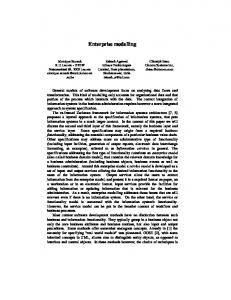
As discussed earlier, a number of landslide squares are characterized as unconditionally unsafe (i.e. for the given parameter values, the squares fail at the start of the simulation). As part of the calibration procedure, these squares were eliminated from the simulation by excluding all landslides which occurred in the first 24 h of the simulation. Figure 6 compares the 50-year map of observed landslides with the upper and lower simulated bounds for 1994–1999. Considering in particular the upper simulated bound, reproduction of the observed spatial distribution is very good, accounting both for areas observed to have landslides and areas observed not to have landslides: for example, the simulation reproduces the observation that, in the northwest half of Valsassina, landsliding is rather more prevalent on the southwest side of the valley than on the northeast side. For the lower simulated bound, the forest root cohesion is too large to allow landsliding in the forested areas and the simulated landslides are therefore on the pasture land. This is not entirely realistic as observation shows that shallow landslides do occur in the forested area. The result suggests that root cohesion, while effective in setting general bounds, is quite a blunt instrument with which to account for detailed spatial distribution. Although the aim was not to reproduce the observed numbers of landslides, the bound values of 369 and 10 661 for the six-year simulation period may be compared with the observed value of 1446 for the fifty-year period. These values give mean annual rates of 61 to 1780 landslides per year for
the simulation compared with an observed rate of 29 landslides per year. If in reality the rate of landsliding is constant, this would suggest that even the lower simulation bound is an overestimate, by about two times. However, it is possible that the six-year test period saw a disproportionate amount of landsliding. There was, for example, a major landslide event at the lower end of Valsassina during the night of 27/28 June 1997. The lower bound may therefore be generally representative of reality. As with previous applications, the upper simulation bound is a considerable overestimate of the observed number but is helpful in defining the spatial distribution of landslides. The landslide model may be predisposed to provide a slight overestimate of the number of landslides owing to the way in which the landsides are counted. The number is calculated as the number of subgrid elements which are simulated as failing. If two neighbouring elements fail they are counted as two separate slides, whereas in reality they may have been one. On the basis of these results, the landslide model is considered to be representative of Valsassina. However, the lower bound on landsliding is likely to be rather closer to the observed incidence than is the upper bound. 5.4
Sediment yield calibration
For the simulations, uncertainty bounds were set on the soil erodibility coefficients for raindrop impact and overland flow (Eqs. 4 and 5) (Table 2) while hydrological input was pro-
198
J. C. Bathurst et al.: Scenario modelling of basin-scale, shallow landslide sediment yield
Table 3. Results forfor thethe SHETRAN Table 3 Results SHETRANValsassina Valsassinasimulations. simulations Scenario
Mean annual rainfall
Mean annual potential evapotranspiration
Simulated mean annual runoff
Simulated sediment yield
Simulated number of landslides
mm
mm
mm
without landslides t ha-1 yr-1
from landslides only t ha-1 yr-1
total with landslides t ha-1 yr-1
Current climate (1994–1999): - current vegetation - forested hills
1476
873
885
3.05 – 4.95
0.01 – 2.64
3.06 – 7.59
369 – 10661
1476
873
841
1.31 – 1.43
0 – 4.09
1.31 – 5.52
0 – 9923
Future climate (2070–2099) - current vegetation - forested hills
1001
982
470
1.10 – 1.30
0.01 – 0.68
1.11 – 1.98
296 – 9027
1001
982
420
0.43
0 – 2.05
0.43 – 2.48
0 - 8020
lute magnitudes of the simulation results may involve errors vided by the baseline run. From the experience of the field but it is assumed that, when comparing results from different visit, the proportion of ground protected from raindrop or simulations, the directions of change and the relative amount raindrip erosion by vegetation or other cover for the forest, of change are the same as if there were no errors. As above, pasture and rock squares was set at 0.9, 0.9 and 0.7, respecthe hydrological response is simulated for the baseline contively. (For the rock squares, the cover is effectively the exditions (modified to account for the land use change as apposed rock itself.) In addition a loose rock cover fraction propriate) while the landslide and sediment yield simulations of 0.25 was set for the rock squares (Eqs. 4 and 5). Withincorporate uncertainty based respectively on root cohesion out the contribution from debris flows, the resulting sediment yield bounds simulated for 1994–1999 were 3.05–4.95 t ha−1 26 and soil erodibility coefficients. yr−1 for the Pioverna outlet (Table 3). Adding the debris flow 6.1 Scenario generation contribution raises the Pioverna sediment yield to 3.06–7.59 t ha−1 yr−1 , where the yield bounds are modified according to The climate scenario was developed using data from the UK the contributions of the lower and upper bounds on the numHadley Centre global circulation model HadRM3. Monthly ber of simulated landslides. These yields are within the range values of rainfall and potential evaporation were extracted observed for the northeastern Italian Alps (1–10 t ha−1 yr−1 ) from the HadRM3 output for the grid square relevant to Valbut a little higher than the value for the Piemonte catchment sassina for the period 2070–2099 as the future climate and (1–3 t ha−1 yr−1 ). On this basis the sediment yield simufor the period 1960–1990 as a control, representative of the lations are considered to be representative of Valsassina, alrecent past climate. These data were provided by the ECthough possibly they may be a slight overestimate. funded WRINCLE project (WRINCLE, 2004). A UniverNoting that the lower bound on the number of simulated sity of Newcastle stochastic procedure for generating continlandslides is likely to be more realistic than the upper bound, uous time series of rainfall based on the Neyman-Scott model the same is likely to be true for the simulated sediment yield. (Cowpertwait, 1995; Cowpertwait et al., 1996) was paramThis suggests that the supply of material derived from shaleterized using the observed 1990s rainfall data. A check low landslides to the main channel network contributes relshowed that its output statistics for rainfall remained simiatively little to the overall long term sediment yield, comlar to the statistics for the observed rainfall. The stochastic pared with channel and other hillslope erosion processes −1 −1 −1 −1 scheme was then applied to the monthly HadRM3 monthly (only 0.01 t ha yr out of the total of 3.06 t ha yr ). data to generate 100-year time series of hourly rainfall for the two scenario periods. For HadRM3 to be accepted as a reliable basis for the generation of a future climate, it must 6 Scenario simulations be shown to represent also the current (or control) conditions accurately. However, significant differences were found beOnce the full model had been tested for current conditions, it tween the mean annual rainfalls for the generated control was used to explore the sensitivity of the landslide sediment time series of rainfall and for the observed 1990s rainfall. supply system to possible future changes in climate and land Possibly the HadRM3 model was not able to reproduce acuse. It is assumed that any simulation deficiencies apparent curately the variations in rainfall associated with the mounin the calibration will affect the scenario results also but that tain terrain of the Valsassina region. The absolute values of comparison of results between simulations, showing changes rainfall derived from HadRM3 could not therefore be used relative to the current conditions, will be valid. I.e. the abso-
0
20
40
60
80 100 120 140 160 180 200 220 240 260 280 300 320 340 360
Number of days of the year for which discharge is exceeded Fig. 5. Comparison of the normalized flow duration curves measured for the Lambro and Brembo J. C. Bathurstrivers et al.:with Scenario modelling of basin-scale, landslide yield at Bellano the simulated baseline curve and shallow uncertainty boundssediment for the Pioverna
199
Fig. 6. Comparison of uncertainty bounds for the SHETRAN simulation (upper diagrams) with the 50year map of observedbounds landslides (lower diagram) in the Valsassina/Esino Landslide are Fig. 6. Comparison of uncertainty for the SHETRAN simulation (upper diagrams)basin. with the 50-yearlocations map of observed landslides shown dots (lower diagram) in theas Valsassina/Esino basin. Landslide locations are shown as dots.
with confidence. It was assumed, though, that the ratio of the generated future and control rainfalls was a good guide to the change in climate likely to take place over the next hundred years. The mean monthly values of rainfall for the future climate were therefore calculated by multiplying the observed 1990s rainfall by the ratio. The stochastic model was then reparameterized using the revised statistics for future rainfall and rerun to provide a new 100-year time series. The procedure was repeated to generate a time series of data for the current or control period, using the statistics for the observed 1990s rainfall. It was noted that the NeymanScott model tends to overestimate the number of dry days in a year (i.e. without rainfall). The number of dry days in the input statistics for the model was therefore decreased by calibrating the mean monthly statistics for the generated control scenario against the statistics for the observed rainfall: the resulting percentage decrease was then applied also to the future scenario. HadRM3 potential evaporation data were extracted for the periods 1990–1999 (the control period) and 2080–2089 (for the future climate). Mean annual potential evaporation for the control data (520 mm) was low compared with the observed value (873 mm). Consequently the value of 982 mm
used for the future climate is likely to be an underestimate. However, it is used here on the grounds that it was obtained by a clearly defined and objective procedure. In the simulations, potential evaporation is constant through each month (and equal to the mean monthly value), applied pro rata as an hourly value. Through the above procedure, one hundred years of rainfall data were generated and strictly the simulations should be run with this full time series to provide a statistically correct representation of conditions for 2070–2099. However, time constraints did not allow the long simulation times required. The 100 years of rainfall data were therefore split into ten consecutive decades and the mean monthly values determined for each decade. Comparison was then made between the decades and with the corresponding data for the current period. This indicated that all the decades showed a significant and similar change in rainfall pattern compared with the current conditions. That decade which was a rough average of the other decadal monthly distributions was then chosen for simulation. Relative to the current period, mean annual rainfall decreases but within this context winter rainfall increases slightly. Mean annual potential evapotranspiration increases. The relevant figures are shown in Table 3.
200
J. C. Bathurst et al.: Scenario modelling of basin-scale, shallow landslide sediment yield
The most realistic future land use change in Valsassina is for the hillslope meadows to be abandoned and to revert to (or be planted with) forest. The catchment was therefore modelled with the current hillslope meadows replaced by forest: the scenario is extreme but enables the maximum impact to be modelled. 6.2
Scenario results
The climate and land use change scenarios were run separately, to show the effect of the single change relative to current conditions. In addition, the two scenarios were combined, to show the effect of the land use change under an altered climate. In other words, simulations with the current vegetation cover and with forested hillslopes were each carried out for both the current climate and the future climate. The results of the scenario simulations are shown in Table 3. Simulation uncertainty bounds are shown as appropriate. For the future climate with current vegetation, runoff is reduced relative to the current conditions, corresponding to the decrease in rainfall and increase in evaporation. Sediment yields derived from erosion by raindrop impact and sediment yield are likewise reduced. However, the number of landslides shows only a small decrease. This is thought to be because the future climate still has sufficient amounts and intensities of rainfall to cause landsliding near to the current rate of occurrence. Overall sediment yields (including the contribution from landslides) fall, probably because of a reduction in the transport of eroded soil caused by a reduction in overland flow and stream flow. The change to fully forested hillslopes for the current climate produces a small reduction in runoff, resulting from the interception and transpiration of the additional trees. The correspondingly drier soils and the stronger root cohesion in the former hillslope meadows also produce a small reduction in landslide occurrence. Sediment yield is reduced but this is probably due more to a reduction in the transport of eroded soil caused by the reduction in overland flow and stream flow than to the reduction in landslides. Indeed, the upper bound on the contribution of landslide material to the total sediment yield is larger for the fully forested hillslopes than for the current vegetation (4.09 versus 2.64 t ha−1 yr−1 ). This is because the landslide model is so designed that all landslides on forested slopes evolve into debris flows whereas on grass slopes such evolution occurs only under certain restricted conditions (Burton and Bathurst, 1998). Thus, conversion of pasture to forest can increase the number of landslides which evolve into debris flows, allowing more landslide material to be injected directly into the channel network and thereby allowing the sediment yield derived from landslides to increase. Landslides on pasture may simply deposit material on the hillslope, whence it can reach the channel only by being washed in by overland flow. The combination of forested hillslopes and future climate generally enhances the above effects: runoff, sediment yield in the absence of landslides and the number of landslides are reduced to their lowest magnitudes. Compared with the
scenario for future climate and current vegetation, the upper bound on the landslide sediment yield is again higher (2.05 versus 0.68 t ha−1 yr−1 ) and causes the overall sediment yield also to be higher (2.48 versus 1.98 t ha−1 yr−1 ). The scenario results can be explained in terms of model design and capability. In other words they are physically realistic, within the limitations of the model design and scenario characteristics. However, given the uncertainties in the scenario formulation and parameter evaluation, the relative variations between the simulations are likely to be more reliable than the simulated output magnitudes. Comparison of the scenario results with the simulation for the current period therefore provides an indication of the potential future changes in catchment response and thus provides a context within which guidelines for land management can be developed to minimize debris flow impacts. In particular: – for both scenarios, there is only a modest reduction in shallow landslide occurrence and the resulting sediment yield; – assuming that the lower bounds on sediment yield are more realistic than the upper bounds, the supply of shallow landslide material to the channel contributes relatively little to the overall catchment sediment yield; – there is a possibility that an increase in the hillslope forest cover could increase the number of landslides which evolve into debris flows and thus supply sediment directly to the channel network; however, despite the resulting increase in landslide sediment yield, the overall sediment yield would still fall. In other words Valsassina is unlikely to see an increase in shallow landslide incidence in the near to medium future and any current schemes for mitigating sediment yield impact do not therefore require any change of design capability.
7
Conclusions
The social and economic impacts of landsliding and the associated sediment production can be immense. There is a need, therefore, for models which can be used to predict the effects of proposed basin management strategies and of possible future changes in basin characteristics on landslide incidence and sediment yield, in support of more efficient land use planning and engineering design. The application of SHETRAN to the Valsassina focus catchment has addressed this need: (i) Application of the SHETRAN landslide model to the Valsassina focus catchment demonstrates an ability to simulate the observed long term spatial distribution of debris flows and to determine catchment sediment yield within the range of observations from a wider region. However, the annual rate of landsliding may be overestimated even by the lower uncertainty bound.
J. C. Bathurst et al.: Scenario modelling of basin-scale, shallow landslide sediment yield (ii) The scenario applications show that the model can be used to explore the sensitivity of the landslide sediment supply system to changes in catchment characteristics, in particular giving shallow landslide occurrence and sediment yield response as a function of climate and land use. For both scenarios there is a modest reduction in shallow landslide occurrence and the resulting sediment yield relative to simulated current conditions. This suggests that any existing schemes for mitigating sediment yield impact in Valsassina do not require any change of design capability. Further, as the supply of material derived from shallow landslides to the main channel network is responsible for only a small component of the overall catchment sediment yield, the emphasis of such schemes should be on other pathways for transfer of sediment into the main system. Such pathways may include overland flow washing sediment into the channels, local gully erosion and bank erosion. Material stored along the channel network itself is also a significant source of sediment. A number of aspects which require further improvement have also been highlighted. (i) The model initially predicts a large number of unconditionally unsafe landslide squares and an objective means of eliminating these from the main simulation needs to be identified. In this case elimination of such squares was achieved by excluding all landslides which occurred in the first 24 h of the simulation. The method is simple and convenient but retains an arbitrary component in the choice of the 24-h limit. In the application of SHETRAN to the Llobregat catchment, Bathurst et al. (in press) carried out a preceding simulation with specified rainfall characteristics to identify landslides which should have occurred prior to the event of interest and which could thus be excluded from subsequent consideration. This introduces an element of physical reasoning and is a pragmatic approach useful when simulating large events but it involves a degree of calibration. Further exploration of the problem is therefore needed. (ii) The simulated upper bound on the number of landslides is typically a large overestimate of the observed number and means of reducing this need to be investigated. One contributory cause may be that the model defines landslides at the scale of individual pixels. When neighbouring pixels fail they are counted as individual landslides when in fact they may be one single landslide. As the upper bound involves a large number of neighbouring pixel failures, a weighting scheme (perhaps based on observed landslide magnitudes) could be introduced to see if it produced a more appropriate count of actual landslides. (iii) Although root cohesion as a parameter is effective for setting general bounds on landslide occurrence, it is quite a blunt instrument with which to account for
201
detailed spatial distribution. The relative effects of other parameters (including local topographic variation) therefore need to be defined, while the limits on root cohesion values need to be refined for a range of vegetation types. More generally, the Valsassina application has demonstrated a technique for assessing shallow landslide occurrence and the resulting catchment sediment yield on a quantitative basis. The SHETRAN landslide model may therefore be useful in investigating the sensitivity of the landslide sediment supply system to changes in catchment characteristics, in supporting planning decisions and in managing land use to mitigate hazard and to maintain environmental quality in mountain areas. As a catchment scale model, it is relevant to the development of plans for sustainable basin management. Acknowledgements. The authors thank G. B. Crosta, P. Frattini and F. Agliardi (University of Milan-Bicocca) and A. Carrara (Consiglio Nazionale delle Ricerche – Istituto di Elettronica e di Ingegneria dell’Informazione e delle Telecomunicazioni, CNR-IEIIT, Bologna) for their great help in providing data and other information on Valsassina and in supporting the field visit. They also thank the Servizio Azienda Speciale di Sistemazione Montana (Trento) and the Lombardy Region Geological Survey (Milan) for their advice and for their interest in the simulation results. C. Hunt (Technician, University of Newcastle upon Tyne) is thanked for his help and advice in the laboratory analysis of the soil samples. The DAMOCLES project was funded by the Environment and Sustainable Development Programme of the European Commission Research Directorate General, under Contract Number EVG1-CT-1999-00007, and this support is gratefully acknowledged. The paper has benefited significantly from the reviews of P. Frattini and V. D’Agostino. Edited by: G. B. Crosta Reviewed by: V. D’Agostino and P. Frattini
References Abernethy, B. and Rutherfurd, I. D.: The distribution and strength of riparian tree roots in relation to riverbank reinforcement, Hydrol. Process., 15, 63–79, 2001. Anselmo, V., Di Nunzio, F., and Maraga, F.: Rainfall, runoff and sediment supply variability from a small basin field data, Geophysical Research Abstracts (European Geophysical Society), 5, No. 14487, 2003. Bathurst, J. C. and O’Connell, P. E.: Future of distributed modelling: the Syst`eme Hydrologique Europ´een, Hydrol. Process., 6, 265–277, 1992. Bathurst, J. C., Crosta, G., Garc´ıa-Ruiz, J. M., Guzzetti, F., Lenzi, M. and R´ıos, S.: DAMOCLES: Debrisfall Assessment in Mountain Catchments for Local End-users. Proc. 3rd Intl. Conf. Debris-Flow Hazards Mitigation: Mechanics, Prediction and Assessment, edited by: Rickenmann, D. and Chen C-L., Millpress, Rotterdam, Netherlands, 2, 1073–1083, 2003. Bathurst, J. C., Ewen, J., Parkin, G., O’Connell, P. E., and Cooper, J. D.: Validation of catchment models for predicting land-use and climate change impacts, 3. Blind validation for internal and outlet responses, J. Hydrol., 287, 74–94, 2004.
202
J. C. Bathurst et al.: Scenario modelling of basin-scale, shallow landslide sediment yield
Bathurst, J. C., Burton, A., Clarke, B. G., and Gallart, F.: Application of SHETRAN basin-scale, landslide sediment yield model to Llobregat basin, Spanish Pyrenees, Hydrol. Process., in press, 2005. Benda, L. and Dunne, T.: Stochastic forcing of sediment supply to channel networks from landsliding and debris flow, Wat. Resour. Res., 33, 2849–2863, 1997. Beven, K. J.: Rainfall-Runoff Modelling: The Primer, Wiley, Chichester, UK, 360 pp., 2001. Beven, K. and Binley, A.: The future of distributed models: model calibration and uncertainty prediction, Hydrol. Process., 6, 279– 298, 1992. Bowels, J. E.: Engineering Properties of Soils and their Measurement, McGraw-Hill, New York, 2nd edition, 1978. Brath, A. and Franchini, M.: La valutazione regionale del rischio di piena con il metodo della portata indice, in: La Difesa Idraulica dei Territori Fortemente Antropizzati, edited by: Maione, V. and Brath, A., BIOS, Cosenza, Italy, 31–60, 1998. British Standards Institution: British standard methods of test for soils for civil engineering purposes, Part 2 – Classification tests, British Standard BS1377, British Standards Institution, London, 1990a. British Standards Institution: British standard methods of test for soils for civil engineering purposes, Part 7 – Shear strength tests (total stress), British Standard BS1377, British Standards Institution, London, 1990b. Burton, A. and Bathurst, J. C.: Physically based modelling of shallow landslide sediment yield at a catchment scale, Environ. Geol., 35, 89–99, 1998. Chatwin, S. C. and Smith, R. B.: Reducing soil erosion associated with forestry operations through integrated research: an example from coastal British Columbia, Canada, in: Erosion, Debris Flows and Environment in Mountain Regions, Intl. Ass. Hydrol. Sci., Publ. No. 209, CEH-Wallingford, Oxon, UK, 377–385, 1992. CORINE: The CORINE land cover database, http://dataservice.eea. eu.int/dataservice/metadetails.asp?id=188, 2004. Cowpertwait, P. S. P.: A generalized spatial-temporal model of rainfall based on a clustered point process, Proc. Roy. Soc. Lond., Series A, 450, 1995, 163-175. Cowpertwait, P. S. P., O’Connell, P. E., Metcalfe, A. V., and Mawdsley, J. A.: Stochastic point process modelling of rainfall, II. Regionalisation and disaggregation, J. Hydrol., 175, 47–65, 1996. Craig, R. F.: Craig’s Soil Mechanics, 6th edition, Spon Press, Taylor and Francis Group, London, 1997. Crosta, G. B. and Frattini, P.: Distributed modelling of shallow landslides triggered by intense rainfall, Nat. Haz. Earth Sys. Sci., 3, 81–93, 2003, SRef-ID: 1684-9981/nhess/2003-3-81. Denmead, O. T. and Shaw, R. H.: Availability of soil water to plants as affected by soil moisture content and meteorological conditions, Agronomy J., 54, 385–390, 1962. Dhital, M. R.: Causes and consequences of the 1993 debris flows and landslides in the Kulekhani watershed, central Nepal. Proc. 3rd Intl. Conf. Debris-Flow Hazards Mitigation: Mechanics, Prediction and Assessment, edited by: Rickenmann, D. and Chen C.-L., Millpress, Rotterdam, Netherlands, 2, 931–942, 2003. EUROPA: The EU Water Framework Directive – integrated river basin management for Europe, http://europa.eu.int/comm/ environment/water/water-framework/index en.html, 2004.
Ewen, J. and Parkin, G.: Validation of catchment models for predicting land-use and climate change impacts, 1. Method, J. Hydrol., 175, 583–594, 1996. Ewen, J., Parkin, G., and O’Connell, P. E.: SHETRAN: distributed river basin flow and transport modeling system, Proc. Am. Soc. Civ. Engrs., J. Hydrologic Engrg., 5, 250–258, 2000. Gianotti, R. and Montrasio, A.: Foglio 17 Chiavenna, in: Carta Tettonica delle Alpi Meridonali alla Scala 1:200 000, edited by: Castellarin, A., Consiglio Nazionali delle Ricerche, Rome, 1981. Guzzetti, F., Carrara, A., Cardinali, M., and Reichenbach, P.: Landslide hazard evaluation: a review of current techniques and their application in a multi-scale study, Central Italy, Geomorphol., 31, 181–216, 1999. Hicks, D. M., Gomez, B., and Trustrum, N. A.: Erosion thresholds and suspended sediment yields, Waipaoa River Basin, New Zealand, Wat. Resour. Res., 36, 1129–1142, 2000. Holmes, M. G. R., Young, A. R., Gustard, A., and Grew, R.: A region of influence approach to predicting flow duration curves within ungauged catchments, Hydrol. Earth Sys. Sci., 6, 4, 721– 731, 2002, SRef-ID: 1607-7938/hess/2002-6-721. Kessel, M. L.: Timber harvest, landslides, streams, and fish habitat on the Oregon Coast, J. Forestry, 83, 10, 606–607, 1985. L´opez, J. L., Perez, D., and Garc´ıa, R.: Hydrologic and geomorphic evaluation of the 1999 debris-flow event in Venezuela, Proc. 3rd Intl. Conf. Debris-Flow Hazards Mitigation: Mechanics, Prediction and Assessment, edited by: Rickenmann, D. and Chen C.-L.: Millpress, Rotterdam, Netherlands, 2, 989–1000, 2003. Lukey, B. T., Sheffield, J., Bathurst, J. C., Hiley, R. A., and Mathys, N.: Test of the SHETRAN technology for modelling the impact of reforestation on badlands runoff and sediment yield at Draix, France, J. Hydrol., 235, 44–62, 2000. Montgomery, D. R., Sullivan, K., and Greenberg, H. M.: Regional test of a model for shallow landsliding, Hydrol. Process., 12, 943–955, 1998. Preston, N. J. and Crozier, M. J.: Resistance to shallow landslide failure through root-derived cohesion in east coast hill country soils, North Island, New Zealand, Earth Surf. Process. Landf., 24, 665–675, 1999. Saxton, K. E., Rawls, W. J., Romberger, J. S., and Paperdick, R. I.: Estimating generalized soil-water characteristics from texture, Soil Sci. Soc. Am. J., 50, 1031–1036, 1986. Shaw, E. M.: Hydrology in Practice, 3rd edn., Chapman and Hall, London, 1994. Sidle, R. C., Pearce, A. J., and O’Loughlin, C. L.: Hillslope stability and land use, Water Resources Monograph Series 11, American Geophysical Union, Washington DC, 1985. Siena, L.: Modelli distribuiti per la valutazione della pericolosita’ da frane superficiali: analisi del Bacino del T. Esino, Thesis (Tesi di Laurea), University of Milan-Bicocca, Milan, Italy, 2001. Van Genuchten, M. Th.: A closed form equation for predicting the hydraulic conductivity of unsaturated soils, Soil Sci. Soc. Am. J., 44, 892–898, 1980. Ward, T. J., Li, R.-M., and Simons, D. B.: Use of a mathematical model for estimating potential landslide sites in steep forested basins, in: Erosion and Sediment Transport in Pacific Rim Steeplands, Intl. Ass. Hydrol. Sci. Publ. No. 132, CEH-Wallingford, Oxon, UK, 21–41, 1981. WRINCLE: Water Resources: Influence of Climate Change in Europe, http://www.ncl.ac.uk/wrincle, 2004.