Scene Text Recognition Using Part-Based Tree-Structured ...

2013 IEEE Conference on Computer Vision and Pattern Recognition

Scene Text Recognition using Part-based Tree-structured Character Detection Cunzhao Shi, Chunheng Wang, Baihua Xiao, Yang Zhang, Song Gao and Zhong Zhang State Key Laboratory of Management and Control for Complex Systems, CASIA, Beijing, China {cunzhao.shi,chunheng.wang,baihua.xiao,yang.zhang,song.gao,zhong.zhang}@ia.ac.cn

Abstract Scene text recognition has inspired great interests from the computer vision community in recent years. In this paper, we propose a novel scene text recognition method using part-based tree-structured character detection. Different from conventional multi-scale sliding window character detection strategy, which does not make use of the character-specific structure information, we use part-based tree-structure to model each type of character so as to detect and recognize the characters at the same time. While for word recognition, we build a Conditional Random Field model on the potential character locations to incorporate the detection scores, spatial constraints and linguistic knowledge into one framework. The final word recognition result is obtained by minimizing the cost function defined on the random field. Experimental results on a range of challenging public datasets (ICDAR 2003, ICDAR 2011, SVT) demonstrate that the proposed method outperforms stateof-the-art methods significantly both for character detection and word recognition.

1. Introduction

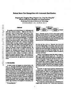
Figure 1. Summary of the proposed word recognition method. Given a text image, we first use tree-structured models to get the character detection results, based on which we get the potential character locations. We then build the CRF model on the potential locations. Character detection scores are used to define the unary cost and language model is used to define the pairwise cost. We finally infer each label of the node and the word by minimizing the cost function.

With the rapid growth of camera-based applications readily available on smart phones and portable devices, understanding the pictures taken by these devices semantically has gained increasing attention from the computer vision community in recent years. Among all the information contained in the image, text, which carries semantic information, could provide valuable cues about the content of the image and thus is very important for human as well as computer to understand the scenes. As proved by Judd et al. [7], given an image containing text and other objects, viewers tend to fixate on text, suggesting the importance of text to human. In fact, text recognition is indispensable for a lot of applications such as automatic sign reading, language translation, navigation and so on. Thus, understanding scene text is more important than ever. Most of the previous work on scene text recognition could be roughly classified into two categories: tradition-

al Optical Character Recognition (OCR) based and object recognition based. For traditional OCR based methods [2, 22, 12], various binarization methods have been proposed to get the binary image which is directly fed into the off-the-shelf OCR engine. However, since text in natural images differs from text in traditional scanned document in terms of resolution, illumination condition, size and font style, the binarization result is usually unsatisfactory. Moreover, the loss of information during the binarization process is almost unrecoverable, which means if the binarization result is poor, the chance of correctly recognizing the text is quite small. As shown in Figure 2, the binarization result is very disappointing, making it almost impossible for the following segmentation and recognition. On the other hand, object recognition based methods assume that scene character recognition is quite simi-

1063-6919/13 $26.00 © 2013 IEEE DOI 10.1109/CVPR.2013.381

2959 2961

acter detection and word recognition. Experimental results are given in Section 3 and conclusions are drawn in Section 4.

2. The Proposed Method 2.1. System Overview Figure 1 shows the flowchart of the proposed method. First, we use part-based tree-structured models to detect characters, based on which we get the potential character locations. Then we build the CRF model on the potential locations. We use character detection scores, spatial constraints and language model to define the unary and pairwise cost function. Finally we get the word recognition result by minimizing the cost function. Next, we will detail the character detection method and word recognition model.

Figure 2. Some scene text binarization results using Otsu [14]. As we can see, the binarization results are quite disappointing, making it difficult for the following segmentation and recognition.

lar to object recognition with a high degree of intraclass variation. For scene character recognition, these methods [4, 13, 19, 18] directly extract features from original image and use various classifiers to recognize the character. While for scene text recognition, since there are no binarization and segmentation stages, most existing methods [19, 18, 11, 10] adopt multi-scale sliding window strategy to get the candidate character detection results. As sliding window strategy does not make use of the special structure information of each character, it will produce many false positives. Thus, these methods heavily rely on the postprocessing methods such as pictorial structures [19, 18] or CRF [11, 10] to choose the final word from piles of candidate detections. When humans try to recognize scene characters with distortions and complex background, the detection of the character from complex background and the recognition of the character are somehow interdependent. On one hand, the unique structure of each character helps us to detect the characters from complex background and on the other hand, detecting the character-specific structure from complex background also helps us to recognize the character. In other words, humans naturally combine detection and recognition together when recognizing characters from scene images. Thus, in this paper, we try to imitate human perceptual ability and propose to recognize characters by detecting character-specific part-based structures, which seamlessly combine detection and recognition together. As both the global structure information and the local appearance information contribute to the part-based tree-structured models for characters, the detection results contain less false positives and thus are more reliable. To recognize the scene text, we build the CRF model on the potential character locations. Character detection scores, spatial constraints and linguistic knowledge are used to define the unary and pairwise cost function. The final word recognition result is acquired by minimizing the cost function. We evaluate our method on a range of challenging datasets (ICDAR 2003, ICDAR 2011, SVT). Experimental results show that our method outperforms state-of-the-art methods considerably. The rest of the paper is organized as follows. Section 2 details the proposed method, including the model for char-

2.2. Character Detection using Part-based Treestructured Models Structure-based model, which captures the local appearance properties and the deformable configuration of an object, has inspired great interest from computer vision community, since Felzenszwalb and Huttenlocher [6] proposed the pictorial structures framework for object recognition. Recently, Zhu and Ramanan [20] proposed to jointly address the tasks of face detection, pose estimation, and landmark localization using mixtures of trees with a shared pool of parts. Although their model is only trained with hundreds of faces, it compares favorably to commercial systems trained with billions of examples. Structure information is even more important to characters, since characters are designed by human and each type of character has unique structure representing itself. To utilize the unique structure information of characters, we model each character as a tree whose nodes correspond to parts of the character. Thus, both the global structure information and the local appearance information are incorporated into the tree-structured model so as to detect the characterspecific structures. Next, we will give details about the model, the inference and the learning. 2.2.1 Model We build a tree-structure based model for each type of character. Figure 3 shows the models for some characters. Each rectangle corresponds to a part-based filter of the character and the red lines illustrate the topological relations of the parts. Model for each character: We represent each character by a tree Tk = (Vk , Ek ), where k is the index of the model for different structures, Vk represents the nodes and Ek specifies the topological relations of nodes [20]. Each node represents a part of the character. Let I represents 2962 2960

Figure 4. Some detection and recognition results. The red rectangle labels the position of the root node of the tree while the blue ones label other parts. The character in the green rectangle labels the type of the sturcture. (a) Detection results of characters with contamination and deformation. (b) Detection results of text images after applying NMS.

Figure 3. Our tree-structured models for some characters. Red lines denote the topological relations of the parts and each rectangle corresponds to a part-based filter.

the input image and li = (xi , yi ) denotes the location of part i. Then the score of the configuration of all the parts L = {li , i ∈ Vk } could be defined as: S(L, I, k) = SApp (L, I, k) + SStr (L, k) + αk where SApp (L, I, k) =



wik · φ(I, li )

2.2.2

(1) (2)

Inferring the character-specific structure corresponds to maximizing S(L, I, k) in (1) over L and k. Since the models are independent from each other, we could maximize S(L, I) for all the structures in parallel. Thus, for each structure, we need to maximize S(I, L) over L:

(3)

S ∗ (I) = max S(I, L)

i∈Vk

and SStr (L, k) =



k wij · ψ(li − lj )

Inference

(4)

L

ij∈Ek

Since each structure Tk = (Vk , Ek ) is a tree, the maximization for each structure could be done efficiently with dynamic programming [20]. We omit the message passing equations for a lack of space. Re-scoring: Apart from unique structure, different parts of a character tend to have similar intensity, which we could utilize to further improve the performance. Thus, we rescore each model by considering the intensity consistency of each part to the root part:

As we can see, the total score of a configuration L for model k consists of the local appearance score in (2), the structure or shape score in (3), and the bias αk . Next, we will give details about the appearance model and the shape model. Local appearance model: Eq. (2) is the local appearance model which reflects the suitability of putting the part based models on the corresponding positions. wik represents the filter or the model for part i, structure k, and φ(I, li ) denotes the feature vector extracted from the location li . Thus, the score of placing part wik on position li is actually the filter response of template wik . We choose HOG [3] as the local appearance descriptor due to its good performance on many computer vision tasks. Global structure model: Eq. (3) is the structure or shape model which scores the character-specific global structure arrangement of configuration L. Here we set ψ(li − lj ) = [dx dx2 dy dy 2 ], where dx = xi − xj and dy = yi − yj are the relative distance from part i to part j. Each term in the sum acts as a spring that constrains the relative spatial positions between a pair of parts. The k , which are learned in the training process, parameters wij could control the location of each part relative to its parent and the rigidity of each spring. By incorporating the elastic structure information, the model could detect characters with contamination or deformation as shown in Figure 4(a).

Snew (L, I, k) = S(L, I, k) +

N 

δ · γdisi,1 ,

(5)

i=2

where N refers to the number of parts, disi,1 is the feature distance between part i and root part. γ is set to 0.2 by crossvalidation. When disi,1 is above a certain value (set to 1.1), δ = 1 if part i is designed to be different from the root part and δ = −1 otherwise. We choose histogram feature to reflect intensity consistency. 2.2.3

Learning

For each type of character, we construct a tree-structured model. To learn the model, we assume a fully-supervised paradigm, where we are provided positive images with characters as well as part labels, and negative images with2963 2961

Then we define a cost function E : Cn → R, to map any labeling to a real number E(·). The function E(·) is defined as a sum of unary and pairwise terms as follows:

out characters. Both the shape and appearance parameters are discriminatively learned using a structured prediction framework. First we need to define the topological structure Ek for each model. We design the tree-structure for each type of character by our experience and the experimental results show that they perform quite well. We give more details in the supplementary material. For a certain type of structure k, given labeled positive examples {In , Ln , kn } and negative examples {In }, we define a structured prediction objective function similar to the one proposed in [21]. Let’s write zn = (Ln , kn ). Note that the scoring function in (1) is linear in model parameters (w, α). Concatenating these parameters into a single vector β, then we could write the score as: S(I, z) = β · Φ(I, z)

E(x) =

n 

Ei (xi ) + λ

i=1



Eij (xi , xj ),

(8)

{i,j}∈N

where x = {x1 , x2 , ..., xn } represents the set of all the random variables, Ei (xi ) is the unary cost function, Eij (xi , xj ) denotes the pairwise cost, and N represents the set of all the neighboring pairs of nodes, which is determined by the structure of the graphical model defined upon them. λ is a tradeoff parameter between the unary and pairwise cost and is set to 0.8 by cross-validation in the experiment.

(6)

Now we would learn a model of the following form: arg min

β,ξn ≥0

 1 β·β+C ξn 2 n

s.t. ∀n ∈ pos β · Φ(In , zn ) ≥ 1 − ξn ∀n ∈ neg, ∀z β · Φ(In , z) ≤ −1 + ξn

2.3.1 Graph Construction After applying Non-Maximum Suppression (NMS) [20] on the original character detection results, the left detection windows constitute the potential locations. We set the overlap parameter for NMS to 0.4 in the experiment. Then, for each location, we choose those detection windows which are close to this location as the candidate characters for this location. We add one node for each potential location sequentially from left to right. The nodes are connected by edges. Since nodes which are spatially distant from each other would not be directly related, we only connect nodes which are close to each other. Figure 1 shows the process.

(7)

The above constraint states that positive examples should score better than 1 (the margin), while negative examples, for all configurations of part positions and structures, should score less than −1. The objective function penalizes violations of these constraints using slack variable ξn . The optimization of the above objective function is a quadratic program (QP). We use the dual coordinate descent solver [5] to solve the problem.

2.3. The Word Recognition Model

2.3.2 Cost Function

Although the character detection step provides us with a set of windows containing characters with high confidence as shown in Figure 4(b), inevitably it also produces some false positives and ambiguities between similar characters. Thus, we need to make use of other information, such as language model and spatial constraints to eliminate these ambiguities. To this end, we build a CRF model on these detection windows. We make use of character detection scores, spatial constraints, and linguistic knowledge to define the cost function. Finally, the word recognition result is acquired by minimizing the cost function. For a given scene text image, there are several potential character locations. Let n be the total number of potential locations. Each position, which might have several character detection results, is represented by a random variable Xi . Since the potential locations might not have any character, we introduce a non-character label to represent these false positives. Thus, each random variable Xi takes a label xi ∈ C = C ∪ { }. We use Cn to represent the set of all possible labeling assignments to all the random variables.

The unary cost E(xi ) represents the penalty of assigning label cj to node xi . In this case, if the detection score for a certain type of character model cj is very high, the cost of labeling the node cj should be small and vise versa. If the scores of all the candidate detections are very low, it is likely for the node to take a null label . To this end, we define the unary cost as follows:  Ei (xi = cj ) =

1 − p(cj |xi ) maxj p(cj |xi )

if cj = , otherwise

(9)

where p(cj |xi ) is the probability for node xi to take label cj . Here we use the detection scores to reflect the confidence for the class. If some character models, e.g., the models for classes {ck , cm }, do not detect the character-specific structures at the position, we set the cost of labeling the node {ck , cm } to a constant 10. We use the pairwise cost function E(xi , xj ) to incorporate linguistic knowledge and spatial constraints. The pairwise cost of two neighboring nodes (xi , xj ) taking labels 2964 2962

(ci , cj ) is defined as: ⎧ 1 − P (ci , cj ) ⎪ ⎪ ⎨ Dij + μ · Si Eij (xi , xj ) = Dij + μ · Sj ⎪ ⎪ ⎩ Dij + μ · Si,j

3.1. Datasets

= = , = = (10) where P (ci , cj ) refers to the bi-gram language model learnt from the lexicon, Dij is the relative distance of the two nodes, Si and Sj represent the maximum character detection scores at the corresponding locations, Si,j is the larger one of Si and Sj , and μ is set to 1.5 in the experiment. We use the SRI Language Modeling Toolkit [17] to learn the probability of joint occurrences of characters in a large English dictionary with around 0.5 million words provided by authors of [10]. The pairwise cost function means that if the probability of joint occurrence of a character pair (ci , cj ) is large, the cost of nodes (xi , xj ) taking labels (ci , cj ) should be small. Moreover, if the relative distance of the two nodes is small, and the maximum score of the node is low, the cost of the node taking a null label should be small. 2.3.3

if ci if ci if ci if ci

= ∧ cj = ∧ cj = ∧ cj = ∧ cj

Character recognition datasets. To evaluate the performance of the proposed detection based character recognition method, we test the recognition rate on two public datasets: Chars74k [4] and ICDAR 2003 robust character recognition dataset (ICDAR03-CH) [9]. However, since we focus on detecting and recognizing characters with certain structures, characters with similar structures such as, ’0’, ’O’ and ’o’, ’P’ and ’p’, ’K’ and ’k’, ’X’ and ’x’, should belong to the same class. Thus, in total, we have 49 types of structures to detect and recognize. To make full use of the whole test set which contains 62 classes, we combine the samples from classes with similar structures to form a new class. We choose training samples for all the structures from Chars74k dataset. The number of training samples varies from 10 to 30 and once the final structure based model for each class is trained, they are used on all the tasks. For chars74k dataset, all the remaining images except those chosen as training samples comprise the test set. While for ICDAR03-CH dataset, since we do not use the training set to learn the model parameters, we evaluate the performance on both the training and test sets. In total, we have 6148, 5835, and 5245 test samples for Chars74k, ICDAR03-CHTrain and ICDAR03-CH-Test respectively. Word recognition datasets. We use the challenging public datasets Street View Text (SVT) [19], ICDAR 2003 robust word recognition [9] and ICDAR 2011 word recognition datasets [16] to evaluate the performance of the overall word recognition method. The SVT dataset contains images taken from Google View Street. Since we focus on the word recognition task, we use the SVT-WORD dataset following the experimental protocol of [19, 18]. For ICDAR 2003 and ICDAR 2011 datasets, similar to [18], we ignore words with less than two characters or with non-alphanumeric characters.

Inference

After computing the unary and pairwise cost, we use the sequential tree-reweighted message passing (TRW-S) algorithm [8] to minimize the cost function in (8), due to its efficiency and accuracy on our recognition problem. The TRW-S algorithm maximizes a concave lower bound on the energy. It begins by considering a set of trees from the random field and computes probability distributions over each tree, which are then used to reweight the messages being passed during loopy BP [15] on each tree. The algorithm terminates when the lower bound cannot be increased further, or the maximum number of iterations has reached. To conclude, given a scene text image, we first (1) use the tree-structured model for each type of character to detect possible characters; (2) then use these detection windows to decide the potential character locations on which the CRF model is defined; (3) compute the unary and pairwise cost function based on the detection scores, the spatial constraints and the language model; and (4) finally infer the most likely word using the TRW-S algorithm.

3.2. Detection Based Character Recognition To recognize characters using the detection model, we apply each character-specific tree-structured model (TSM) on the image and choose the structure with the highest score as the recognition result. Apart from the recognition results of the first candidate, we also evaluate recognition results with candidate number varying from 2 to 5. Similar to most methods [13, 19, 18], we choose “HOG+KNN ”as the benchmark method. Concretely, each image is partitioned into 4 × 3 blocks, from which we extract HOG [3] features, and KNN is used to recognize the character. The recognition results on Chars74k, ICDAR03-CH-Train and ICDAR03-CH-Test are shown in Figure 5. The results show that the proposed TSM outperforms HOG+KNN more than 10% on ICDAR03-CH dataset, when only considering the first candidate. When increasing the candidate number to 2, we find that the performance of

3. Experimental Results In this section, we give detailed evaluation of the proposed character detection and word recognition method. We compare the detection based character recognition method with conventional HOG+NN. We also compare the proposed character detection method with conventional sliding window strategy, SYNTH+FERNS proposed by Wang et al. [18]. For word recognition task, we compare our results with state-of-the-art methods [19, 18, 10, 11] as well as commercial OCR engines ABBYY FineReader 9.0 [1]. 2965 2963

(a) Chars74k dataset(%)

(b) ICDAR03-CH-Train dataset(%)

(c) ICDAR03-CH-Test dataset(%)

Figure 5. Character recognition results with different candidate number on different datasets. Since we focus on detecting characters with unique structures, we only train 49 types of character model whose structures are different from each other. Thus the recognition results are reported on 49 classes.

Method ICDAR03(FULL) ICDAR03(50) SVT

TSM improves more quickly with an increase of about 8% whereas the recognition rate of HOG+KNN only increases 3%-5%. The great improvement suggests (1) the effectiveness of the tree-structured models, as they tend to detect and recognize characters with certain structures, and thus (2) the high possibility of achieving better recognition result if we postprocess the result to deal with similar structures. When we consider the recognition rates of the first 5 candidates, the result is quite encouraging, reaching 86.38%, 91.88%, 89.74% on Chars74k, ICDAR03-CH-Train and ICDAR03CH-Test respectively. Since all the training samples are chosen from Chars74k dataset, the results further demonstrate that, for the proposed method, the model trained on one dataset could generalize well on other datasets.

FERNS+PLEX [18] 62 76 57

TSM+PLEX 70.47 80.70 69.51

Table 1. Word recognition results using word spotting strategy PLEX. For FERNS+PLEX, multi-scale sliding window strategy is used to detect characters and FERNS classifier is used to recognize the characters. While for TSM, tree-structured models are used to detect and recognize the characters at the same time. Both methods adopt the same postprocessing strategy PLEX.

strategy to detect and recognize characters, which does not make use of the character-specific global structure information. Thus, there are many false positives, which would disturb the word spotting stage. While for the proposed character detection method, since we make use of both global structure information and local appearance information, the detection results are more reliable and representative.

3.3. Character Detection To evaluate the superiority of the proposed character detection method over conventional multi-scale sliding window detection strategy for word recognition, we test the word recognition result using the word spotting strategy PLEX from [18]. In this case, based on the character detection results of the proposed TSM and the SYNTH+FERNS proposed by Wang et al. [18], same postprocessing strategy PLEX is used to find the final word. Similar to [18], for ICDAR 2003, we measure performance using a lexicon created from all the words that appear in the test set (we call this ICDAR03(FULL)), and with lexicons consisting of the ground truth words for that image plus 50 random words added from the test set (we call this ICDAR03(50)). In the SVT-WD case, a lexicon of about 50 words is provided with each image as part of the dataset. The word recognition results are shown in Table 1. The results demonstrate that TSM+PLEX outperforms FERNS+PLEX considerably on all the tasks. Since we use the same word spotting strategy PLEX, the only difference between the two methods lies in the character detection method. Wang et al. [18] used multi-scale sliding window

3.4. Word Recognition To recognize the word, we build the CRF model on the character detection results as discussed in Section 2.3. We add one node for each potential location and nodes are connected based on their horizonal spatial distance. We use ICDAR 2003, ICDAR 2011 and SVT datasets to evaluate the proposed word recognition method. Same bigram language model learnt from the lexicon with 0.5 million words is used on all the datasets. Similar to the evaluation scheme in [18] and [11], we use the inferred result to retrieve the word with the smallest edit distance in the lexicon. For ICDAR datasets, we measure performance using a lexicon created from all the words in the test set (ICDAR03(FULL), ICDAR11(FULL)), and with lexicon consisting of the ground truth words plus 50 random words from the test set (ICDAR03(50), ICDAR11(50)). For SVT dataset, we use the lexicon provided by Wang et al. [18]. We compare our methods with state-of-the-art

2966 2964

Figure 6. Examples of word recognition results of the proposed method. Our method could recognize scene text with low resolution, different fonts and distortions.

Method ABBYY9.0 [1] SYNTH+PLEX [18] TSM+PLEX Method in [11] Method in [10] Our method

ICDAR03(FULL) 55 62 70.47 67.79 79.30

ICDAR03(50) 56 76 80.70 81.78 81.78 87.44

ICDAR11(FULL) 74.23 82.87

ICDAR11(50) 80.25 87.04

SVT 35 57 69.51 73.26 73.26 73.51

Table 2. Word recognition rates of the proposed method and recent state-of-the-art methods on ICDAR 2003, ICDAR 2011 and SVT. The results on ICDAR03(50), ICDAR11(50), SVT are acquired by retrieving the ones with the smallest edit distance in the lexicon of 50 words whereas for ICDAR03(FULL) and ICDAR11(FULL), the lexicon contains all the ground truth words in the test set.

methods [18, 11, 10] and the results are shown in Table 2. The results show that our method constantly performs better than state-of-the-art methods on all the tasks. The proposed method outperforms TSM+PLEX by 6%-9%, showing the effectiveness of the CRF model which incorporates detection scores, linguistic knowledge and spatial constraints, since both methods adopt the same character detection method. Our method also outperforms the approach proposed by Mishra et al. [11, 10] by more than 10% on ICDAR03(FULL). Note that Mishra et al. also used the CRF model to encode character detection results and language model. However, they used the multi-scale sliding window strategy to get the candidate character locations and SVM to classify these characters. The detection method is not as good as the proposed tree-structured character detection method which makes use of the intrinsic global structure information. Furthermore, they built the CRF model on all the detection windows as long as their spatial distance and overlap ratio satisfy a certain condition, which makes the CRF model more complex than ours since we only use the potential character locations to define the nodes. What’s more, Mishra et al. [11] computed the node-specific lexicon prior for each text image from their corresponding lexicon, which means (1) the lexicon priors heavily rely on the lexicon for that image and (2) the computation cost is increased since the lexicon prior should be recomputed for each image. On the contrary, we use the same bi-gram language model learnt from a large dictionary with 0.5 million words on all the tasks. This further demonstrates the generalization ability and the adaptivity

Figure 7. Examples from SVT that our method failed to recognize.

of the proposed method. Compared to [11], the recognition rates on SVT do not improve a lot, mainly because some of the scene text images in SVT are difficult to recognize even for human as shown in Figure 7. We also report recognition results on ICDAR11 dataset (ICDAR11(FULL) and ICDAR11(50)) for future comparison. Some of the recognition results from ICDAR and SVT are shown in Figure 6. As we can see, our method could recognize scene text with low resolution, different fonts and distortions. The reasons that our method achieves an increase in recognition rates of more than 10% on ICDAR03(FULL) and 6% on ICDAR03(50) mainly lie in: (1) the part-based tree-structured character detection model makes use of the global structure information and the local appearance information, seamlessly combining character detection and recognition together; and (2) we integrate the detection scores, spatial constraints and language model into the carefully designed CRF model so that different types of information could be optimally balanced. Both the character detection and word recognition are implemented in Matlab. The average processing time to recognize a scene text image is about 3 seconds on an In2967 2965

tel(R) Core(TM) i7-2600 CPU 3.40GHZ processor. Since the character detectors are independent from each other, the implementation could be much faster using parallel processing.

[6] P. Felzenszwalb and D. Huttenlocher. Pictorial structures for object recognition. International Journal of Computer Vision, 61(1):55–79, 2005. [7] T. Judd, K. Ehinger, F. Durand, and A. Torralba. Learning to predict where humans look. In IEEE 12th International Conference on Computer Vision (ICCV), pages 2106–2113. IEEE, 2009. [8] V. Kolmogorov. Convergent tree-reweighted message passing for energy minimization. IEEE Transactions on Pattern Analysis and Machine Intelligence, 28(10):1568 – 1583, 2006. [9] S. Lucas, A. Panaretos, L. Sosa, A. Tang, S. Wong, and R. Young. Icdar 2003 robust reading competitions. In Proceedings of the Seventh International Conference on Document Analysis and Recognition (ICDAR), volume 2, pages 682– 687, 2003. [10] A. Mishra, K. Alahari, and C. V. Jawahar. Scene text recognition using higher order langauge priors. In BMVC, 2012. [11] A. Mishra, K. Alahari, and C. V. Jawahar. Top-down and bottom-up cues for scene text recognition. In Proceedings of IEEE Conference on Computer Vision and Pattern Recognition(CVPR), 2012. [12] L. Neumann and J. Matas. Real-time scene text localization and recognition. In Proceedings of IEEE Conference on Computer Vision and Pattern Recognition (CVPR), 2012. [13] A. Newell and L. Griffin. Multiscale histogram of oriented gradient descriptors for robust character recognition. In International Conference on Document Analysis and Recognition (ICDAR), pages 1085–1089. IEEE, 2011. [14] N. Otsu. A threshold selection method from gray-level histograms. Automatica, 11:285–296, 1975. [15] J. Pearl. Probabilistic reasoning in intelligent systems: Networks of plausible inference. Morgan Kauffman, 1988. [16] A. Shahab, F. Shafait, and A. Dengel. Icdar 2011 robust reading competition challenge 2: Reading text in scene images. In International Conference on Document Analysis and Recognition (ICDAR), pages 1491–1496. IEEE, 2011. [17] A. Stolcke et al. Srilm-an extensible language modeling toolkit. In Proceedings of the international conference on spoken language processing, volume 2, pages 901–904, 2002. [18] K. Wang, B. Babenko, and S. Belongie. End-to-end scene text recognition. In International Conference on Computer Vision (ICCV), 2011. [19] K. Wang and S. Belongie. Word spotting in the wild. Computer Vision–ECCV, pages 591–604, 2010. [20] Z. Xiangxin and D. Ramanan. Face detection, pose estimation, and landmark localization in the wild. pages 2879 – 2886, 2011. [21] Y. Yang and D. Ramanan. Articulated pose estimation with flexible mixtures-of-parts. In IEEE Conference on Computer Vision and Pattern Recognition (CVPR), pages 1385–1392. IEEE, 2011. [22] M. Yokobayashi and T. Wakahara. Segmentation and recognition of characters in scene images using selective binarization in color space and gat correlation. In Proceedings. Eighth International Conference on Document Analysis and Recognition (ICDAR), pages 167–171. IEEE, 2005.

4. Conclusion In this paper, we propose an effective scene text recognition method using the CRF model to incorporate treestructure based character detection and linguistic knowledge into one framework. Different from the conventional multi-scale sliding window character detection strategy, which does not make use of the intrinsic global structure information, we propose to learn a part-based tree-structured model for each type of character to detect and recognize the characters simultaneously. Based on these detection results, we build a CRF model on the potential character locations to integrate detection scores, spatial constraints and language model. We report results on three of the most challenging datasets and the results show that our method not only outperforms the most popular work published at ICCV 2011 [18] significantly but also improves the latest results published by Mishra et al. [11, 10] considerably. The experimental results show that our method could recognize text in unconstrained scene images with a high accuracy. This could greatly help us in building systems, such as scene understanding, automatic sign reading, language translation, navigation and so on.

Acknowledgment We thank the anonymous reviewers for their valuable comments and suggestions. This work was supported by the National Natural Science Foundation of China (NSFC) under Grants No. 60933010, No. 61172103 and No. 61271429 and National High-tech R&D Program of China (863 Program) under Grant No. 2012AA041312.

References [1] Abbyy finereader 9.0. http://www.abbyy.com. [2] X. Chen and A. Yuille. Detecting and reading text in natural scenes. In Proceedings of IEEE Conference on Computer Vision and Pattern Recognition (CVPR), volume 2, pages II– 366. IEEE, 2004. [3] N. Dalal and B. Triggs. Histograms of oriented gradients for human detection. In IEEE Conference on Computer Vision and Pattern Recognition (CVPR), volume 1, pages 886–893, 2005. [4] T. de Campos, B. Babu, and M. Varma. Character recognition in natural images. In VISAP, 2009. [5] P. Felzenszwalb, R. Girshick, D. McAllester, and D. Ramanan. Object detection with discriminatively trained partbased models. IEEE Transactions on Pattern Analysis and Machine Intelligence, 32(9):1627–1645, 2010.

2968 2966