Publié par : Published by : Publicación de la :
Faculté des sciences de l’administration Université Laval Québec (Québec) Canada G1K 7P4 Tél. Ph. Tel. : (418) 656-3644 Fax : (418) 656-7047
Édition électronique : Electronic publishing : Edición electrónica :
Aline Guimont Vice-décanat - Recherche et partenariats Faculté des sciences de l’administration
Disponible sur Internet : Available on Internet Disponible por Internet :
http ://www.fsa.ulaval.ca/rd
[email protected]
DOCUMENT DE TRAVAIL 2001-003 SCHEDULING A SINGLE MACHINE WITH SEQUENCE DEPENDENT SETUP TIME USING ANT COLONY OPTIMIZATION. Caroline Gagné, Wilson L. Price, Marc Gravel
Version originale : Original manuscript : Version original :
ISBN – 2-89524-123-6 ISBN ISBN -
Série électronique mise à jour : One-line publication updated : Seria electrónica, puesta al dia
04-2001
Scheduling a single machine with sequence dependent setup times using Ant Colony Optimization Caroline Gagné (1), Wilson L. Price (1) Département d’informatique et mathématique, Université du Québec, Chicoutimi, Québec, G7H 2B1
(2)
& Marc Gravel (1)
(2) Faculté des sciences de l’administration, Université Laval, Québec, Québec, G1K 7P4
Abstract We describe an Ant Colony Optimization (ACO) algorithm for solving a single machine scheduling problem. In the operating situation modeled, setup times are sequence dependent and the objective is to minimize total tardiness. This problem has previously been treated by Rubin & Ragatz [1995] and by Tan et al. [2000] among others. A new feature using look-ahead information in the transition rule of the ACO algorithm shows an improvement in performance. A comparison with other solution approaches indicates that the ACO that we describe is competitive and has a certain advantage for larger problems. Keywords : scheduling, metaheuristic, ant colony optimization, single machine, total tardiness, sequence dependent setups.
1. Introduction Industrial production scheduling constitutes a fertile field for both researchers and practitioners of operational research. The interest in this field is generated not only by the problem-solving challenge that it offers but also by the practical results that can be achieved. However, researchers such as Maccarthy & Liu [1993] and McKay & Wiers [1999] have remarked on the sometimes wide gap between the theoretical problems treated and those met in practice. The development of efficient solution procedures for the scheduling of orders in a casting center belonging to a Canadian multinational firm is the principal aim of the research reported in this paper. The authors have previously reported [Gravel et al., 2000] [Gravel et al., 2001] details of successful work in this metaheuristics area. The aim of this paper is to report on the performance of some extensions to the "ant colony optimization" (ACO) algorithm [Dorigo, 1992] which has already demonstrated its usefulness in this industrial situation and is presently incorporated in software used by the firm. In the industrial application, the holding furnaces may require certain draining and cleaning operations of varying durations between the casting of two successive orders for different metal alloys. These operations may be seen as the setup operations dealt with in the literature. We seek a schedule for current released orders that takes into account these sequence dependent setup times as well as multiple objectives. We validate the performance of the new elements that we have introduced by solving a known problem from the literature, the single machine problem with sequence dependent setups. This allows us to compare our results with those previously published [Tan et al., 2000] for various metaheuristics. Single machine scheduling is a classic problem that has been well covered in the literature [Koulamas, 1997]. This problem offers a lower level of complexity than that of other configurations often treated in scheduling publications, such as parallel and serial machines, or cellular shops. It is, however, possible to achieve interesting practical results through the study of single machine shops. For example, some shops may have a bottleneck machine that strongly influences performance and which therefore allows the shop to be studied as a single machine
Scheduling a single machine with sequence-dependent …;
C. Gagné, W.L. Price, M. Gravel
[Graves, 1981] [Hax & Candea, 1984]. We have already referred to our own workon an application treating complex operations having sequence dependent setup times as a single machine shop. Various objective functions may be useful in the scheduling of a single machine shop. Among these, we find the minimization of total tardiness, an objective that seeks to improve customer service. Meeting target delivery dates has been declared as the most important scheduling objective by Wisner & Siferd [1995] who also found that 58% of production planners actively seek to meet delivery dates. Even in the case of a single machine, minimizing tardiness is a difficult objective to attain since there are no simple sequencing rules that apply, save in two cases described by Emmons [1969], and in these two cases, the setups are sequence independent. In general, the problem of scheduling a single machine with sequence dependent setup times has generally been presented with the objective of minimizing the total production time (makespan) for the set of released orders [Baker, 1992] [Morton & Pentico, 1993]. In this case, the problem may be represented as a traveling salesman problem. Where the objective is to meet delivery dates where setup times are sequence dependent, the literature is not extensive. One of the conclusions of Allahverdi et al. [1999] is that there is a need for further research in this area, and in scheduling in general. Formally, the problem of scheduling a single machine having sequence dependent setup times where the objective is the minimization of total tardiness can be defined as follows [Rubin & Ragatz, 1995]: let there be n jobs to produce, all released at time zero, and which must be completed without interruption on a single machine. Each job j has as attributes its production duration pj, its delivery date dj, and its setup time sij, which is incurred when job j is undertaken following job i in an job sequence Q. We define Q = {Q(0), Q(1), …, Q(n)} as the job sequence where Q(j) is the subscript of the jth job in the sequence and where Q(0) = 0. The machine is continuously available through the planning period and can process only one job at a time. Once a job is started it must be completed without interruption. The end time of job j is expressed as: j
cQ(j) = ∑ [sQ(k −1)Q(k) + pQ(k) ] . k =1
The tardiness for this same job j is expressed as:
tQ(j) = max{ 0, cQ(j) − dQ(j)}. The objective to be minimized is the total tardiness T for the set of jobs to be produced and is expressed as: n
TQ = ∑ tQ(j). j =1
Previous authors such as Ragatz [1993], Rubin & Ragatz [1995] and Tan & Narasimhan [1997] proposed a branch and bound algorithm for this problem as well as a genetic algorithm, a local improvement method and a simulated annealing algorithm. In this paper we present an ant colony optimization heuristic which has certain advantages for this case. In particular, it allows us to use various elements of information about the problem to better direct the search for good solutions. Moreover, the basic algorithm has already demonstrated its capacity to perform well in comparison to other metaheuristics in an industrial setting [Gravel et al., 2001]. Our objective was to improve on this performance on the one hand by including extensions suggested in the literature, and on the other through the use of new 2
Scheduling a single machine with sequence-dependent …;
C. Gagné, W.L. Price, M. Gravel
elements that use broader information in the transition rule. The validation of the effectiveness of this metaheuristic in solving the single machine scheduling problem described will be presented in terms of the solution quality and the computation times. We compare our results to those reported in a recent study by [Tan et al., 2000]. A brief review of the single machine scheduling literature is offered in the following section. 2. Literature survey The single machine scheduling problem with constant or zero setup times has been well covered in the literature. Koulamas [1994] presents a review of the total tardiness minimization problem and points out that many solution approaches are available for the single machine problem. He proposes a classification of the proposed methods as optimal or heuristic. The first class includes dynamic programming, branch and bound and hybrids including both. The author points out that dynamic programming algorithms are superior and that the most efficient method was proposed by Potts & Van Wassenhove [1982]. The class of heuristic methods can be further broken down to sub-classes including constructive algorithms, local search methods and decomposition methods. Results indicate that local search and decomposition approaches are generally more effective than construction heuristics. Two major theoretical developments must be pointed out concerning the single machine scheduling tardiness-minimization problem. Emmons [1969] developed the dominance condition and several authors [Lawler, 1977] [Potts & Van Wassenhove, 1982] wrote on subject of the decomposition principle. These contributions allowed the development of optimal solution procedures but they also inspired the construction of various heuristics [Della Croce et al., 1998]. Adding the characteristic of sequence dependent setup times, however, increases the complexity of the problem of minimizing total tardiness on a single machine. This characteristic invalidates the dominance principle as well as the decomposition principle [Rubin & Ragatz, 1995]. Du & Leung [1990] seem to have been the first to show that this problem is NP-hard. The importance of explicitly treating sequence dependent setups in production scheduling has been pointed out a number of times in the literature. In particular Wilbrecht & Prescott [1969] state that this is particularly where production equipment is being used close to its capacity levels. Wortman [1992] states that the efficient management of production capacity requires the consideration of setup times. The papers of Panwalkar et al. [1973], Flynn [1987] and Krajewski et al. [1987] also refer to this question. From a practical point of view, many industrial situations require the explicit consideration of setups and the development of appropriate scheduling tools. Previous authors have described cases highlighting this situation. Pinedo [1995] describes the situation of a manufacturing plant making paper bags where setups are required when the type of bag changes. The duration of a setup depends on the similarity of the bags made in the preceding lot. A similar situation was observed in the plastics industry by Das et al. [1995] and Franca et al. [1996]. The printing industry also has setups that are sequence dependent because various cleaning operations are required when the print colors are changed [Conway et al., 1967]. The aluminum industry has casting operations where setups, mainly affecting the holding furnaces, are required between the casting of different alloys [Gravel et al, 2000]. The textile, pharmaceutical, chemical and metallurgical industries present other practical examples where sequence dependent setups are frequently observed. 3
Scheduling a single machine with sequence-dependent …;
C. Gagné, W.L. Price, M. Gravel
Despite the copious literature in scheduling, it was only in 1999 that two reviews of problems with sequence dependent setups were published [Allahverdi et al., 1999] [Yang & Liao, 1999]. These authors have proposed different classifications of the field but arrive at similar conclusions. Allahverdi et al. [1999] point out gaps in existing research, including in the underlying theoretical underpinnings and in the treatment of multiple objectives. The general conclusion of this review is that scheduling where sequence dependent setups are required is a fertile area for further research. Yang & Liao [1999] observe that there are few comparisons of the solution methods developed for this problem. They make the same observation concerning the applications of the various methods available in practical situations. The literature shows [Allahverdi et al., 1999] that while many industrial applications have sequence dependent setups, few papers have treated this characteristic in combination with the objective of meeting delivery dates. Few authors have treated the problem described in the previous section. Among these Ragatz [1993] proposed a branch and bound algorithm for the exact solution of smaller problems. A genetic algorithm and a local improvement method were proposed by Rubin & Ragatz [1995] while Tan & Narasimhan [1997] tackle this same problem through simulated annealing. Finally Tan et al. [2000] present a comparison of these four approaches and conclude, following a statistical analysis, that the local improvement method offers better performance than simulated annealing, which is turn better than branch and bound. In this comparison, the genetic algorithm had the worst performance. The authors propose an ant colony optimization (ACO) algorithm for the solution of the single machine scheduling problem with sequence dependent setups. This industrial scheduling problem from the aluminum industry consists in the scheduling of a set of released jobs on a casting rig and has been formulated as a single machine with sequence dependent setups and multiple objectives. We found the basic ACO to be effective in terms of solution quality and that it had relatively low computation times [Gravel et al., 2001]. In this paper, we report on the addition of extensions to the basic algorithm and on numerical experiments that compare our results to those found using other metaheuristics. 3. Ant colony optimization (ACO) 3.1 The basic algorithm This metaheuristic was first introduced in the doctoral thesis of Marco Dorigo [1992] and was inspired by the behaviour of real ants [Deneubourg et al., 1983] [Deneubourg & Goss, 1989] [Goss et al., 1990]. Ants communicate through pheromone, a deposit that they leave on the ground in varying intensities as they move about. As more ants use the same path, the more pheromone is deposited. Ants tend to follow these pheromone trails and in this manner, they communicate with each other as to the location of food sources. When an obstacle is placed on an existing path so as to block it, some ants will go about it by the right side, others by the left side. Those having chosen the shortest path will rejoin the previous pheromone trail more quickly. This results in a more rapid buildup of pheromone on the shorter path, and still more ants will be attracted to it. In this way the favored path from a nest to a food source tends to the shortest distance no matter what the first path found may have been. One of the first applications of the ACO was to the solution of the traveling salesman problem (TSP). A matrix D of the distances dij between pairs (i,j) of cities is known, and the objective is to find the shortest tour of all cities. In the application of the ACO to this problem, each ant is seen as an agent with certain characteristics [Dorigo et al., 1991]. First, an ant at city i will 4
Scheduling a single machine with sequence-dependent …;
C. Gagné, W.L. Price, M. Gravel
choose the next city j to visit taking into account both the distance to each of the available choices and of the existing "pheromone" trail. When the ant then moves from city i to city j, it leaves a trail of "pheromone" on edge (i,j). Finally the ant k has a memory that prevents returning to those cities already visited. This memory is referred to as a tabu list, tabuk, and is an ordered list of the cities already visited by ant k. This concept, one should note, is somewhat different from that of the same name proposed by Glover [1989; 1990a,b]. We now describe details of the choice process. At time t the ant chooses the next city to visit considering a first factor called the trail intensity τij(t). The intensity contains information as to the volume of traffic that previously used edge (i,j). The greater the level of the trail, the greater the probability that it will again be chosen by another ant. At the initial iteration, the trail intensity τij(0) is initialized to a small positive quantity τ0. The choice of the next city to visit depends also on a second factor called the visibility, ηij, which is the quantity 1/dij. This visibility acts as a greedy rule that favors the closest cities in the choice process. In making the choice of the next city to visit, the transition rule pijk (t ), allows a trade-off between the trail intensity (edges having had previous heavy traffic) and the visibility (the closest cities). The probability that an ant k will starting from city i will go to city j is given by equation (1) of Figure 1. Coefficients α and β are parameters that allow control of the trade-off between the intensity and the visibility. If the total number of ants is m and the number of cities to visit is n, a cycle is completed when each ant has completed a tour. In the basic version of the ACO, the trail intensity is updated at the end of a cycle so as to take into account the evaluation of the tours that have been found in this cycle. The evaluation of the tour of ant k is called Lk, and will influence the trail quantity ∆τ ijk that is added to the existing trail on the edges (i,j) of the chosen tour. This quantity is proportional to the length of the tour obtained and is calculated as Q/Lk, where Q is a system parameter. The updating of the trail also takes into account a persistence factor ρ (or evaporation factor [1-ρ]). This factor serves to diminish the intensity of the existing trail over time. Therefore the addition to the trail on those edges used by various ants in the current cycle and the evaporation of part of the previous trail determine the trail intensity for the next cycle as shown in the following expression: m
τij (t +1) = ρ ⋅ τ ij(t) + ∑∆τ ijk k =1
where ∆τ ijk =
Q Lk
(2)
3.2 Extensions to the basic algorithm Various extensions to the basic algorithm just presented have been proposed, notably by Dorigo & Gambardella [1997]. The improvements concern the transition rule, the trail updating rules, the use of local improvement rules and the use of a restricted candidate list. These extensions have been included in the algorithm proposed in this article. Transition rule Gambardella & Dorigo [1997] have suggested a modification to the original transition rule described by equation (1). They suggest that the ant at city i should choose the next city j to visit according to the modified rule presented in equation (3) of Figure 1. In this equation, q is a random number and q0 is a parameter; both are between 0 and 1. J represents the value obtained by the original transition rule of equation (1). Parameter q0 determines the relative importance of the exploitation of existing information of the network and the exploration of new solutions. If exploitation is chosen, the next city is determined by the highest value in equation (3) and in the 5
Scheduling a single machine with sequence-dependent …;
C. Gagné, W.L. Price, M. Gravel
case of exploration, the next city is chosen at random using the probabilities computed in (1). The transition rule incorporated in equations (1) and (3) is called the "pseudo-randomproportional rule". Global trail update In the basic algorithm, the trail is updated at the end of a cycle when all ants have completed a tour. The quantity of pheromone to be added to an edge is therefore proportional to the quality of the tour obtained by each ant as shown in equation (2). In the modified scheme, the pheromone trail is updated at the end of a cycle, but only on the edges of the best solution found in the cycle (cycle*). Equation (4) of Figure 1 is used for the global trail update rather than equation (2). In this equation (4), ρg (0 q 0
where J is chosen according to probability: p (t) = k ij
[τ ij(t )]α ⋅ [s1 ]β ⋅ [m1 ]δ α β δ ∑[τil(t )] ⋅ [s1 ] ⋅ [m1 ] ij
l∉Tabouk
ij
il
(1')
il
Local improvement methods We have included two local improvement methods in the ACO algorithm. The first of these two methods is the restricted 3-opt method described by Dorigo & Gambardella [1997]. This method has the important characteristic of not inverting the complete order sequence, which is important where setup times are sequence dependent. The second method, called RSPI (Random Search Pairwise Interchange), proceeds to invert each pair of adjacent orders in turn. This method was used by Rubin & Ragatz [1995] either alone or in conjunction with a metaheuristic to solve the single machine, sequence dependent setup times, minimization of total tardiness problem. The results, presented in Tan et al. [2000] for this problem, indicate that the RSPI offers results that are better than those obtained by simulated annealing, branch and bound and the genetic algorithm if sufficient computation time is allowed. One of these local improvement methods is applied to the path found by each ant. The choice of method is made by a random (fair coin toss) choice. The restricted 3-opt method, in which one cycles only once through the list of adjacent pairs, is applied in order to reduce the computation times, which is particularly important if the problem size is large. Candidate list The use of a candidate list limits the number of choices for the next order to place in the sequence. In the TSP, the candidates chosen are the closest "cities" to the current one. In the scheduling problem treated here, the candidate list is made up of those orders having the smallest slack times. The calculation of the slack for order j, where j∉Tabu, following order i, is done according to the definition of mij in equation (7). The list of orders {j} is then sorted in increasing order of slack and the first cl of these become the candidate list for order i. Parameter values In most cases, the values of the parameters in the ACO algorithm follows the suggestions given by Dorigo & Gambardella [1997] and in the remaining cases, the values have been determined through direct numerical experimentation. The trail is initialized to the value, τ0 = (n⋅Lnn)-1 where n is the size of the problem and Lnn is the result of a solution obtained either randomly or through some simple heuristic. The remaining parameters have been assigned the following 9
Scheduling a single machine with sequence-dependent …;
C. Gagné, W.L. Price, M. Gravel
values: ρg = ρl, = 0.9, m = 10, q0 = 0.9 and cl = 0.3⋅n with a lower bound equal to 10. Further the maximum number of cycles without improvement of the best known solution is fixed at 50. Note that the values of α, β and δ have been adjusted empirically according to the problem characteristics (processing time variance, tardiness factor, due dates range) and take values between 1 and 4. For example, where the due-dates are such that tardiness factor is high, more weight is given to the slack matrix. 4.2 Including look-ahead information While we have included the supplementary improvements suggested by Dorigo & Gambardella [1997], we also propose a new element in the transition rule. Usually, the selection of the next order to place in the sequence is the result of a compromise between the trail, information on past choices, and the visibility, information derived from the problem parameters. In addition, we propose the addition of look-ahead information about the potential of the current partial solution. The idea that we propose differs in a number of respects from that proposed by Michel & Midderdorf [1999] for a different problem. These authors proposed a look-ahead function which works by evaluating the trail intensity resulting from a choice. The look-ahead information that we propose estimates the potential quality of a partial solution by taking the actual value generated by the current partial solution and adding the consequences of one of the candidate choices as well as a lower bound on the remaining uncompleted portion. The computation of the lower bound for the uncompleted portion follows the method used in the branch and bound computations of Ragatz [1993], and later in Tan et al. [2000]. The lower bound on the total tardiness of the partial solution Qh , including the order j presumed to be the candidate chosen following order i, is calculated according to the following:
Bij = TQ h + TQ 'h
(8)
Equations (1') and (3') related to the transition rule are again modified by the addition of a new term, Bij , which represents the look-ahead information. As for the two measures of distance, relative values are used to obtain a comparable scale of values and the parameter φ controls the weight of this information. The lower bound for a partial solution including the candidate order j is therefore divided by the largest bound among the list {j} of candidates. The following definitions are obtained: arg max l∉Tabou k j= J
{[τ (t )] ⋅ [ il
α
1 s il
]β ⋅ [m1 ]δ ⋅ [B1 ]φ } il
il
if q ≤ q0 if q > q0
(3')
where J is chosen according to the probability: p (t) =
[τ ij(t )]α ⋅ [s1 ] β ⋅ [m1 ]δ ⋅ [B1 ]φ β δ φ ∑[τ il(t )]α ⋅ [s1 ] ⋅ [m1 ] ⋅ [B1 ] ij
k ij
l∉Tabou k
and where Bij =
Bij Max Bij
ij
il
ij
il
(1')
il
(9)
The performance of this new element in the ACO algorithm has been studied and is presented in section 6 in performance comparisons with and without the look-ahead information. We show that, while there is an increased computational load imposed by the need to compute the lookahead information, we obtain an improvement in solution quality. 10
Scheduling a single machine with sequence-dependent …;
C. Gagné, W.L. Price, M. Gravel
5. Numerical experiments
A series of numerical experiments allowed us to evaluate the performance of our ACO algorithm and to compare it to previous solution methods. We first compare a version of our ACO method without look-ahead information with a version that incorporates this feature. We then compare our approach to other heuristics previously compared in Tan et al. [2000], including a branchand-bound algorithm, a genetic algorithm, a simulated annealing method and the RSPI local improvement procedure. All tested algorithms used the set of thirty-two test problems devised by Rubin & Ragatz [1995] and available on the Internet at (http://mgt.bus.msu.edu/datafiles.htm). The problem set is divided by size into four groups of problems having 15, 25, 35 and 45 orders respectively. Moreover, the eight problems of each group were derived from a 2x2x2 experimental plan related to three characteristics each of which may be adjusted to one of two levels. These characteristics are the processing time variance (PTV), the tardiness factor (TF) and the due dates range (DDR). The operation times of the orders are normally distributed with an arbitrary mean of 100 units and the setup times are uniformly distributed with a mean of 9.5 units. Each of the problems was solved twenty times both in the results quoted from the work of Tan et al. [2000] and in our ACO algorithm experiments. We worked on two different computers. In an attempt to reproduce as closely as possible the experimental conditions of these latter authors who worked on an Intel Pentium 90-MHz machine, we obtained an Intel Pentium 100-Mhz computer. We were, however, unable to compare other machine characteristics such as the available RAM, and we realise that our comparisons can only be approximate. We completed our experiments by testing our ACO algorithm on a current computer having an Intel Pentium III 733-Mhz processor with 256 Meg RAM, running under Windows 2000. The ACO algorithm is coded in the C language. Note that the algorithms compared in Tan et al.[2000] were coded in different languages. We created a new series of larger test problems having the same characteristics as the original set. These test problems are divided into four groups having 55, 65, 75, and 85 orders respectively. We present the results obtained using our ACO algorithm on these problems in the next section and we will make the problem set available to those wishing to use them in future comparative experiments. 6. Computational results
A first comparison seeks to evaluate the impact on solution quality of the new elements that we have introduced into the transition rule. Table 1 presents the results of two different versions of the ACO for the 32-problem set. Both versions include the modifications to the basic algorithm proposed by Dorigo & Gambardella [1997] but only one includes the look-ahead information previously described. Problems were solved 20 times using each algorithm and the table shows the percentage difference with respect to the best solution found by the branch-and-bound algorithm for the best ACO solution, the median ACO value and the worst ACO solution. The branch-and-bound results are drawn from Tan et al. [2000]. Those branch-and-bound results that are optimal are indicated by an asterisk, and in other cases computation was stopped after a maximum of five million nodes were generated. The first columns of the table show the problem characteristics. For each algorithm, the times shown are the averages of the twenty solution runs. 11
Scheduling a single machine with sequence-dependent …;
C. Gagné, W.L. Price, M. Gravel
From Table 1, we note that, in general, the look-ahead information has allowed an improvement in solution quality. Six exceptions are highlighted (in grey) in the table. In five of these six cases the quality drop is less than 1%. In the remaining case, problem #705, the median value of the gap with the branch-and-bound solution has dropped from 3% to 5.6%. There has been an increase in computation times due to the use of look-ahead information. Generally, as Table 1 shows, solution times have increased by less than a factor of two, although in some instances the increase is higher. Currently, look-ahead information is computed every time the transition rule is used, but we feel that a more selective use of this information would allow us to retain the solution quality improvements while imposing a lesser computational penalty.
Table 1 : Experimental ACO results for 32 problems with and without look-ahead information.@
We analysed our results to determine whether the quality improvements observed have statistical significance. Conover & Iman's [1981] result allows us to use a parametric t-test on the average ranking. The ranking was obtained from the 40 runs of the two algorithm versions for each problem. However, to avoid a too-large number of ties, as is the usual practice, we have fourteen problems where 80% or more of the results are identical have been set aside for this test. Table 2 presents the results of this statistical test which allows us to draw the conclusion that the version of the algorithm that includes look-ahead information offers solutions of better quality. 12
Scheduling a single machine with sequence-dependent …;
C. Gagné, W.L. Price, M. Gravel
The eighteen problems considered by this test are listed in column 1 of Table 1 in bold characters. INCLUDING lookahead information 16.811 98.591 380
WITHOUT lookahead information 24.189 137.741 380
Mean rank Variance Number of cases t value 2-tailed prob.
9.356 0.000
Table 2 : T-TEST for a comparison of two mean rank for the 18 problems considered: two samples with different variances. The significance level for the test is 5%.
These results have encouraged us to conclude that using look-ahead information contributes significantly to improving solution quality and we therefore proceeded to compare this version of the ACO algorithm to the genetic, simulated annealing and RSPI local improvement heuristics and the branch-and-bound algorithm presented in Tan et al. [2000]. Figure 2(a), which is derived from the data of Table 3, shows the percentage difference between the median results of the branch-and-bound algorithm and the different heuristics tested in Tan et al. and provides visual confirmation of the ranking of these methods. The ACO algorithm is compared to the RSPI heuristic in Figure 2(b). Tan et al. [2000] presented a statistical analysis showing that the RSPI method performed better than the other approaches tried and so it is used in the following comparisons with our results.
40.0
150.0
30.0 20.0
100.0
10.0
50.0
0.0 -10.0
0.0
-20.0
(a)
-30.0 RSPI ACO Prob701
Prob601
Prob501
RSPI
Prob401
Prob701
SA Prob601
Prob501
GA Prob401
-50.0
(b)
Figure 2: Percentage difference of the median results for different heuristics vs the B&B results. (a) Performance of the genetic algorithm (GA), simulated annealing (SA) and the RSPI local improvement method. (b) Performance of the RSPI local improvement method and the ant colony optimization (ACO) algorithm.
Table 3 presents the details of the results obtained by the heuristics of Tan et al. [2000] and of our ACO algorithm experiments. The form is similar to that of Table 1 and shows the same three performance indicators.
13
Scheduling a single machine with sequence-dependent …;
C. Gagné, W.L. Price, M. Gravel
Table 3 : Comparison of the performance of the ant colony optimization (ACO) algorithm with the methods reported in Tan et al. [2000] :branch and bound (B&B), genetic algorithm (GA), simulated annealing (SA), and the RSPI local improvement method.@
14
Scheduling a single machine with sequence-dependent …;
C. Gagné, W.L. Price, M. Gravel
The figures highlighted in gray indicate which of the ACO or RSPI methods is better and where performance is rated the same. We note that the smaller problems having 15 and 25 orders are more easily solved by the RSPI. The ACO algorithm has a better solution in only three such cases as compared to 16 for the RSPI. For the 35-order problem group, performance of the two methods is about the same. For the larger problems, the ACO performs better 12 times compared to the RSPI method which is better 6 times. We are observe that the ACO algorithm has a relative advantage for the larger problems. The values of the ACO parameters α, β, δ and φ were set to identical values for all problems having the same characteristics. These parameters were adjusted following empirical tests on the more realistic larger-sized problems. The results of a number of tests allow us to conjecture that the ACO algorithm could have performed better for the small problems had we specifically adjusted the parameters for them. A statistical analysis allowed the confirmation of the summary conclusions that may be drawn from Figure 2. Tan et al. [2000] graciously furnished us with their detailed results to allow this analysis to be made. As in the statistical analysis of Table 2, the problems for which the two heuristics produced 80% or more identical results were ignored to avoid a preponderance of ties. The fourteen problems considered are indicated in column one of Table 3 in bold characters. Table 4 shows the statistical analyses on the average rank grouped by problem size. Because the problems of 15 orders showed little variation in results among methods they were not considered in this analysis. The results of the statistical tests appear in Table 4 and part (a) shows that the RSPI method has the better performance for problems of 25 orders, part (b) indicates that the two heuristics offer equal performance and part (c) shows that for the larger problems, the ACO algorithm is superior. In summary, the statistical analysis confirms our earlier remarks. (a) Mean rank Variance Number of cases t-value 2-tailed prob
ACO 23.85 138.90 40
(b) RSPI 17.15 95.86 40
ACO 21.23 151.78 120
2.766 0.007
(c) RSPI 19.77 114.97 120
0.984 0.326
ACO 17.28 125.42 120
RSPI 23.73 121.99 120 -4.492 0.000
Table 4: T-TEST for a comparison of two mean rank for the 18 problems considered: two samples with equal variances. (a) 2 problems of 25 orders, (b) 6 problems of 35 orders and (c) 6 problems of 45 orders. The significance level for these tests is 5%.
The number of times that a heuristic is superior to another does not, however, convey the degree of difference in performance. For this reason, the average percentage difference for those cases where one method is better than the other has been calculated, using the median results. The RSPI heuristic shows a 2.87% lead over the ACO in cases where it is better, but the ACO has a 13.89% lead over the RSPI in those cases where the ACO is better. Figure 2(b) illustrates this difference in the amplitude of the differences between the two methods. We note, therefore, that using the ACO can produce a much better result than the RSPI but it is not likely to be, even in the worst case, much worse than the RSPI result. Particular cases in the results in Table 3 have been noted: -
the RSPI has better performance for the 8th problem of each group, that problem where PTV is high, TF is moderate and DDR is large;
15
Scheduling a single machine with sequence-dependent …;
-
C. Gagné, W.L. Price, M. Gravel
the largest difference in results is observed for problem #508 between the median and the worst case results.
It is likely that these differences could be lessened were the parameters of the ACO adjusted to the characteristics of these specific problems. In other problems the ACO algorithm produces much better results: -
for the first and fifth problems (those with low TF and close DDR) in the 35 and 45 order problem sets;
-
for the odd numbered 45-order problems of Table 3 (highlighted in gray);
-
for all problems having closely spaced due-dates, the ACO algorithm is better for all three performance measures;
We note that the ACO algorithm uses specific information concerning the setups and the due dates in the form of the two distance matrices and it is, no doubt, this information that allows a greater measure of success in meeting the due dates. Finally the second and the sixth problems of each group proved easy for both solution methods. Table 5 presents further statistical t-test on the mean rank for those problems having the same PTF, TF and DDR characteristics. Again those problems for which 80% of the results are identical have been set aside to avoid a preponderance of ties. The second and sixth problems were also set aside since they were easily solved to optimality by both approaches. Analyses (a), (b) and (d) of Table 5 show that the ACO algorithm is superior for the first, third and fifth problems of each order-size group. Analyses (c), (e) and (f) of Table 5 show the RSPI to perform better for the fourth, seventh and eight problems of each group. In each t-test on mean ranking, a variance comparison test was also used before. (a) Mean rank Variance Number of cases t-value 2-tailed prob
ACO 12.73 83.01 60
(b) RSPI 28.27 55.61 60
ACO 13.88 70.25 40
-10.219 0.000
Mean rank Variance Number of cases t-value 2-tailed prob
ACO 23.75 131.71 60
(f) RSPI 17.25 116.29 60
3.197 0.002
RSPI 13.70 57.33 40 6.443 0.000
(e) RSPI 27.53 55.46 40
-6.797 0.000
ACO 27.30 120.88 40
-6.190 0.000
(d) ACO 13.48 115.44 40
(c) RSPI 27.13 113.01 40
ACO 30.00 53.82 40
RSPI 11.00 33.53 40 12.858 0.000
Table 5 (a), (b), (c), (d), (e) and (f) : T-TEST for a comparison of two mean rank for problems having same characteristics (the nth problem of each group). Note that the 2nd and the 6th problem are not included in this analysis because a lack of variances. The tests (a), (b), (e) and (f) have two samples with equal variances and the tests (c) (d) have two samples with unequal variances. The significance level for these tests is 5%.
We have already pointed out that comparisons of solution times are difficult not only because of the nature of the computers used but also because of the nature of the algorithms. Tan et al. [2000] have used fixed solution times of 6, 16, 30, and 60 minutes for problems of size 15, 25, 35 and 45 orders respectively. The ACO algorithm uses quite different stopping criteria. Despite 16
Scheduling a single machine with sequence-dependent …;
C. Gagné, W.L. Price, M. Gravel
these differences and to further our understanding of the results, we show the average computing time required by the ACO algorithm in the final column of Table 3. In the measure that the results of the two sets of numerical experiments can be compared, we note that the ACO algorithm does not approach the solution times of the RSPI even in the worst cases. For example, the longest solution time for solution of 45 order problems, when run on a 100MHz Pentium computer, is about 44 minutes as compared to the 60 minutes allowed the RSPI. When run on a current computer, solution time for problems of this size was under two minutes as shown in the final column of Table 1. Table 6 presents a statistical analysis similar to the previous ones concerning the equality of mean ranking for the set of fourteen problems retained. Neither algorithm was shown to dominate the other in this test. Mean rank Variance Number of cases t-value 2-tailed prob
ACO 19.911 143.616 280
RSPI 21.089 120.432 280 -1.214 0.225
Table 6 : T-TEST on mean ranking for the 14 problems considered: two samples with equal variances. The significance level for these tests is 5%.
In summary, our statistical tests show that for the Rubin & Ragatz [1995] problem set the ACO algorithm is competitive in solution quality and has shorter computation times than the best performing method tried by Tan et al. [2000]. The RSPI seems to perform somewhat better on small problems while the ACO algorithm is better for the larger problems.
Table 7 : Results for larger test problems (55, 65, 75, 85 orders).@
17
Scheduling a single machine with sequence-dependent …;
C. Gagné, W.L. Price, M. Gravel
A new set of larger test problems were generated randomly using a procedure defined by Ragatz [1993]. These problems are available through the Internet at http://depcom.uqac.uquebec.ca/~c3gagne/. Each problem of 55, 65, 75, and 85 orders was solved 20 times by the ACO algorithm. Table 7 presents the results in the format of the relevant previous tables and adds the mean and standard deviation of the results obtained. We offer these results to provide a basis for future comparisons of larger sized problems more typical of real order books. 7. Conclusions
The single machine scheduling problem with sequence dependent setup times for total tardiness minimization is NP-hard, but we have found that the Ant Colony Optimization algorithm that we have presented is able to efficiently solve problems of a size encountered in industrial situations. The modifications and adaptations of the original ACO algorithm that we propose have contributed to the performance of this method in the cases studied. The generalization of the concept of distance drawn from the TSP to include two distance matrices, one based on setup times and the second on due dates, has proven useful in controlling algorithm performance and might be generalized to allow solution of industrial problems with multiple objectives. The use of look-ahead information in the selection of the next order during the construction of a solution has been shown, with the support of statistical tests, to improve solution quality. The extra computational load does not, in our opinion, lengthen solution times unduly. In an industrial context, the improvements in solution quality will compensate wholly for the longer computational times. The Ant Colony Optimization algorithm described here has performed competitively with the best results obtained by Tan et al. [2000] for other heuristics. Overall, the solutions obtained by the ACO algorithm for larger problems are of equal or better quality and the computational times are appreciably lower. For the smaller problems we did not find this advantage to hold, but such problems are, in our experience, less representative of those found in industry. To better represent these larger problems, we make available a further problem set in the hope that it may be useful to other authors in future numerical experiments. Our results have encourages us to incorporate the ACO algorithm presented in our practical work on the scheduling of aluminum casting. Acknowledgements
This research was financially supported by the FCAR (Québec) and NSERC (Canada) granting councils. The authors also wish to thank Professor Paul A. Rubin and his colleagues for having generously furnished details of their own results and for their valuable comments.
18
Scheduling a single machine with sequence-dependent …;
C. Gagné, W.L. Price, M. Gravel
References
Allahverdi A., Gupta J.N.D., Aldowaisan T., [1999], A review of scheduling research involving setup considerations, Omega, 27, 219-239. Baker K.R, [1992], Elements of sequencing and scheduling, Hanover, NH. Colorni A., Dorigo M., Maniezzo V., [1991], Distributed optimization by ant-colonies, Proceedings of the European Conference on Artificial Life (ECAL'91), Elsevier Publishing, Paris, France, 134-142. Conover W.J., Iman R.L., [1981], Rank transformations as a bridge between parametric and nonparametric statistics, The American Statistician, 35, 124-129. Conway R.W., Maxwell W.L., Miller L.W., [1967], Theory of scheduling, Addison Wesley, MA. Das S.R., Gupta J.N.D., Khumawala B.M, [1995], A saving index heuristic algorithm for flowshop scheduling with sequence dependent set-up times, The Journal of the Operational Research Society, 46, 1365-1373. Della Croce F., Tadei, R., Baracco P., Grosso A., [1998], A new decomposition approach for the single machine total tardiness scheduling problem, The Journal of the Operational Research Society, 49, 10, 1101-1106. Deneubourg J.L., Pasteels J.M., Verhaeghe J.C., [1983], Probabilistic behaviour in ants: A strategy of errors ?, Journal of Theorical Biology, 105, 259-271. Deneubourg J.L., Goss S., [1989], Collective patterns and decision-making, Ethology & Evolution, 1, 295-311. Dorigo M. [1992], Optimization, learning and natural algorithms, Ph.D. Thesis, Politecnico di Milano, Italy. Dorigo M., Di Caro G., [1999], The Ant Colony Optimization Meta-Heuristic, In: D. Corne, M. Dorigo and F. Glover Editors, New Ideas in Optimization, McGraw-Hill. Dorigo M., Gambardella L.M., [1997], Ant colonies for the traveling salesman problem, BioSystems, 43, 73-81. Dorigo M., Maniezzo V., Colorni A., [1991], Positive feedback as a search strategy, Technical Report No 91-016, Politecnico di Milano, Italy, 20 pages. Dorigo M., Maniezzo V., Colorni A., [1996], Ant system: optimization by a colony of cooperating agents, IEEE transactions on System, Man & Cybernitic, 26, 1, 29-41. Du J., Leung J.Y., [1990], Minimizing total tardiness on one machine is NP-hard, Mathematics of Operations Research, 15, 483-494. Emmons H., [1969], One-machine sequencing to minimize certain functions of job tardiness, Operations Research, 17, 701-715. Franca P.M., Gendreau M., Laporte G., Muller F.M., [1996], A tabu search heuristic for the multiprocessor scheduling problem with sequence dependent setup times, International Journal of Production Economics, 43, 79-89. Flynn B.B., [1987], The effects of setup time on output capacity in cellular manufacturing, International Journal of Production Research, 25, 1761-1772. 19
Scheduling a single machine with sequence-dependent …;
C. Gagné, W.L. Price, M. Gravel
Glover F., [1989], Tabu search – Part I, ORSA Journal on Computing, 1, 190-206. Glover F., [1990a], Tabu search – Part II, ORSA Journal on Computing, 2, 4-32. Glover F., [1990b], Tabu search: A tutorial, Interfaces, 20, 4, 74-94. Goss S., Beckers R., Deneubourg J.L., Aron S., Pasteels J.M., [1990], How trail laying and trail following can solve foraging problems for ant colonies, In: Behavioral Mechanisms of Food Selection, R.N. Hughes ed., NATO-ASI Series, vol. G20, Berlin: Springler-Verlag. Gravel M., Price W., Gagné C., [2000], Scheduling jobs in a Alcan aluminium factory using a genetic algorithm, International Journal of Production Research, 38, 13, 3031-3041. Gravel M., Price W., Gagné C. [2001], Scheduling continuous casting of aluminum using a multiple-objective ant colony optimization metaheuristic, Document de Travail, Faculté des Sciences de l’Administration, Université Laval, Québec, Canada. (submitted for publication). Graves S.C., [1981], A review of production scheduling, Operations Research, 29, 646-675. Hax A.C., Candea D., [1984], Production and inventory management, Prentice-Hall Inc., Englewood Cliffs, N.J. Johnson D.S., McGeoch L.A., [1997], The traveling salesman problem: a case study in local optimization, Local Search in Combinatorial Optimization, E.H.L. Aarts & J.K. Lenstra editors, John Wiley and Sons Ltd., pp. 215-310. Kanellakis P.-C., Papadimitriou C.H., [1980], Local search for the asymmetric traveling salesman problem, Operations Research, 28, 5, 1087-1099. Koulamas C., [1994], The total tardiness problem: review and extensions, Operations research, 42, 6, 1025-1041. Koulamas C., [1997], Polynomially solvable total tardiness problems: review and extensions, Omega, 25, 2, 235-239. Krajewski L.J., King B.E., Ritzman L.P., Wong D.S., [1987], Kanban, MRP and shaping the manufacturing environment, Management Science, 33, 39-57. Lawler E.L., [1977], A "pseudopolynomial" algorithm for sequencing jobs to minimize total tardiness, Annals of Discrete Mathematics, 1, 331-342. Lawler E.L., Lenstra J.K., Rinnooy-Kan A.H.G., Shmoys D.B., [1985], The traveling salesman problem, Wiley, New York. Maccarthy B.L., Liu J. [1993], Addressing the gap in scheduling research: a review of optimization and heuristic methods in production scheduling, International Journal of Production Research, 31, 1, 59-79 McKay K.N., Wiers V.C.S., [1999], Unifying the theory and practice of production scheduling, Journal of Manufacturing Systems, 18, 4, 241-255.. Michel R., Middendorf M., [1999], An ACO algorithm for the shortest common supersequence problem, In: D. Corne, M. Dorigo and F. Glover Editors, New Ideas in Optimization, McGraw-Hill. Morton T.E., Pentico D.W., [1993], Heuristic scheduling systems: with applications to production systems and project management, John Wiley & Sons, New York. 20
Scheduling a single machine with sequence-dependent …;
C. Gagné, W.L. Price, M. Gravel
Panwalkar S.S., Dudek R.A., Smith M.L., [1973], Sequencing research and the industrial scheduling problem, Symposium on the Theory of Scheduling and its Applications, Beckmann M., Goos P.G., Zurich H.P.K., ed., 29-38. Pinedo M., [1995], Scheduling theory, algorithms and systems, Prentice-Hall, NJ. Potts C.N., Van Wassenhove L.N., [1982], Decomposition algorithm for the single machine total tardiness problem, Operations Research Letters, 1, 177-181. Ragatz G.L., [1993], A branch-and-bound method for minimum tardiness sequencing on a single processor with sequence dependent setup times, Proceedings: Twenty-fourth Annual Meeting of the Decision Sciences Institute, 1375-1377. Reinelt G., [1994], The traveling salesman: computational solutions for TSP applications, Springler-Verlag, New York. Rubin P.A., Ragatz G.L. [1995], Scheduling in a sequence dependent setup environment with genetic search, Computers and Operations Research, 22, 2, 85-99. Tan K.C., Narasimhan R., [1997], Minimizing tardiness on a single processor with sequence dependent setup times: a simulated annealing approach, Omega, 25, 6, 619-634. Tan K.C., Narasimhan R., Rubin PA., Ragatz G.L., [2000], A comparison of four methods for minimizing total tardiness on a single processor with sequence dependent setup times, Omega, 28, 313-326. Wilbrecht J.K., Prescott W.B., [1969], The influence of setup time on job performance, Management Science, 16, B274-B280. Wisner J.D., Siferd S.P., [1995], A survey of U.S. manufacturing practices in make-to-order machine shops, Production and Inventory Management Journal, 1, 1-7. Wortman D.B., [1992], Managing capacity: getting the most from your firms assets, Industrial Engineering, 24, 47-49. Yang W.-H., Liao C.-J., [1999], Survey of scheduling research involving setup times, International Journal of Systems Science, 30, 2, 143-155.
21