This is the Pre-Published Version
Scheduling Linear Deteriorating Jobs with an Availability Constraint on a Single Machine1 Min Ji
a, b, 2
Yong He
b, 3
T.C.E. Cheng
c, 4
a
College of Computer Science & Information Engineering, Zhejiang Gongshang University, Hangzhou 310035, P.R. China b Department of Mathematics, State Key Lab of CAD & CG, Zhejiang University, Hangzhou 310027, P.R. China c Department of Logistics, The Hong Kong Polytechnic University, Kowloon, Hong Kong
1 This research was supported by the Teaching and Research Award Program for Outstanding Young Teachers in Higher Education Institutions of the MOE, China, and the National Natural Science Foundation of China (10271110, 60021201). The third author was supported in part by The Hong Kong Polytechnic University under a grant from the Area of Strategic Development in China Business Services. 2 Email:
[email protected] 3 Email:
[email protected] 4 Corresponding author. Email:
[email protected]
Abstract We consider a single machine scheduling problem in which the processing time of a job is a simple linear increasing function of its starting time and the machine is subject to an availability constraint. We consider the non-resumable case. The objectives are to minimize the makespan and the total completion time. We show that both problems are NP-hard and present pseudo-polynomial time optimal algorithms to solve them. Furthermore, for the makespan problem, we present an optimal approximation algorithm for the on-line case, and a fully polynomial time approximation scheme for the off-line case. For the total completion time problem, we provide a heuristic and evaluate its efficiency by computational experiments. Keywords. Scheduling; Computational complexity; Approximation algorithms; Deteriorating job; Availability constraint
1
1
Introduction
For most scheduling problems it is assumed that the job processing times are fixed parameters [17], and the machines are available at any time. However, such restrictive assumptions represent an oversimplified view of reality. Job processing times are not necessarily deterministic because jobs may deteriorate while waiting to be processed. Examples can be found in financial management, steel production, resource allocation and national defense, etc., where any delay in processing a job may result in deterioration in accomplishing the job. For a list of applications, the reader is referred to Kunnathur and Gupta [12], and Mosheiov [16]. Such problems are generally known as the deteriorating job scheduling problem. The assumption of the continuing availability of machines may not be valid in a real production situation, either. Scheduling problems with machine availability constraints often arise in industry due to preventive maintenance (a deterministic event) or breakdown of machines (a stochastic phenomenon) over the scheduling horizon. In this paper we will study the deteriorating job scheduling problem with a machine availability constraint due to a deterministic event. Work on the deteriorating job scheduling problem was initiated by Brown and Yechiali [3] and Gupta and Gupta [10]. They focused on the single machine makespan problem under linear deteriorating conditions. Since then, scheduling problems with time-dependent processing times have received increasing attention. An extensive survey of different models and problems was provided by Alidaee and Womer [1]. Cheng, Ding and Lin [5] recently presented an updated survey of the results on scheduling problems with time-dependent processing times. Graves and Lee [9] point out that machine scheduling with an availability constraint is very important but still relatively unexplored. They studied a scheduling problem with a machine availability constraint in which maintenance needs to be performed within a fixed period. Lee [13] presented an extensive study of the single and parallel machine scheduling problems with an availability constraint with respect to various performance measures. Two cases are usually considered for such problems. If a job cannot be finished before the next down period of a machine and the job can continue after the machine becomes available again, it is called resumable. On the other hand, it is called non-resumable if the job has to restart rather than continue. For more details, the reader may refer to Lee, Lei and Pinedo [14]. The problem under consideration can be formally described as follows: There are n independent jobs J = {J1 , J2 , · · · , Jn } to be processed non-preemptively on a single machine which is available at time t0 > 0. Let pj , αj and Cj denote the actual processing time, the growth (or deteriorating) rate and the completion time of Jj , respectively. The actual processing time of job Jj is pj = αj sj , where sj is the starting time of Jj in a schedule. We assume that the machine is not available during the period between time b1 and b2 (which is called the non-available period), where b2 > b1 > t0 . The processing of any job is non-resumable. Let Cmax = max1,···,n {Cj } and Z =
Pn
j=1 Cj
denote
the makespan and the total completion time of a given schedule, respectively. The objectives are
2
to minimize the makespan and the total completion time. Using the three-field notation of [8], we denote these two problems as 1/nr − a, pj = αj sj /Cmax and 1/nr − a, pj = αj sj /
P
Cj , respectively.
Using the same denotation as Lee [13], here nr − a in the second field denotes a non-resumable availability constraint. The above defined problems may date back to Mosheiov [15], who first considered a special case of the problems where the machine is available at any time from t0 . The most commonly used performance measures were considered, such as makespan, total completion time, total weighted completion time, total weighted waiting time, total tardiness, number of tardy jobs, maximum lateness and maximum tardiness. He shows that all these models are polynomially solvable. Chen [4] extended the study to parallel machines, and considered P/pj = αj sj /
P
Cj . He shows that the
problem is NP-hard even with a fixed number of machines. When the number of the machine is arbitrary, he proves that there is no polynomial approximation algorithm with a constant worst-case ratio. He also gives an approximation algorithm with a parameter dependent worst-case ratio for the two machine case. For the problem with a machine availability constraint, Wu and Lee [18] studied the resumable case of the makespan problem, denoted by 1/r − a, pj = αj sj /Cmax . They show that the problem can be transformed into a 0-1 integer program and a linear equation problem. However, the computational complexity of this problem is still unknown. To the best of our knowledge, 1/nr − a, pj = αj sj /Cmax and 1/nr − a, pj = αj sj /
P
Cj are still unexplored.
In scheduling theory, a problem is called on-line (over list) if jobs come one by one in a list, and they are scheduled irrevocably on the machines as soon as they arrive without any information about the jobs that will come later. On the other hand, if we have full information about the jobs before constructing a schedule, the problem is called off-line. Algorithms for on-line and off-line problems are called on-line and off-line algorithms, respectively. The quality of an approximation algorithm is usually measured by its worst-case ratio (for off-line problems) or competitive ratio (for on-line problems), respectively. Specifically, let CA (I) (or briefly CA ) denote the objective value yielded by an approximation algorithm A, and COP T (I) (or briefly COP T ) denote the objective value produced by an optimal off-line algorithm. Then the worst-case ratio (or competitive ratio) of algorithm A is defined as the smallest number c such that for any instance I, CA (I) ≤ cCOP T (I). An on-line algorithm A is called optimal if there does not exist any other on-line algorithm with a competitive ratio smaller than that of A. In this paper we show that both of the problems 1/nr − a, pj = αj sj /Cmax and 1/nr − a, pj = αj sj /
P
Cj are NP-hard and present their respective pseudo-polynomial time optimal algorithms.
Furthermore, for the problem 1/nr − a, pj = αj sj /Cmax , we present an optimal approximation algorithm for the on-line case, and a fully polynomial time approximation scheme for the off-line case. For the problem 1/nr − a, pj = αj sj / by computational experiments.
P
Cj , we provide a heuristic and evaluate its efficiency
3
In the following, we use the symbol [ ] to denote the order of jobs in a sequence. Thus, the actual processing time of the job scheduled in the first position is p[1] = α[1] t0 , and its completion time is C[1] = t0 + p[1] = t0 (1 + α[1] ). Similarly, by induction, the completion time of the job in the jth position is C[j] = C[j−1] + p[j] = t0
2
Qj
i=1 (1
+ α[i] ), if it is processed before the non-available period.
Minimizing the makespan
2.1
NP-hardness
Theorem 1 The problem 1/nr − a, pj = αj sj /Cmax is NP-hard. Proof. We show the result by reducing the Subset Product problem, which is NP-hard [6, 11], to our problem in polynomial time. An instance I of the Subset Product problem is formulated as follows: Given a finite set S = {1, 2, · · · , k}, a size xj ∈ Z + for each j ∈ S, and a positive integer A, does there exist a subset T ⊆ S such that the product of the sizes of the elements in T satisfies Q
j∈T
xj = A?
In the above instance, we can omit the element j ∈ S with xj = 1 because it will not affect the product of any subset. Therefore, without loss of generality, we can assume that xj ≥ 2 for every j ∈ S. Furthermore, we can assume that B =
Q
j∈S
xj /A is an integer since otherwise it can be
immediately answered that there is no solution to the instance. We set D =
Q
j∈S
xj = AB. Then
D ≥ 2k , since every xj ≥ 2. For any given instance I of the Subset Product problem, we construct the corresponding instance II of our problem as follows: – Number of jobs: n = k. – Jobs’ available time: t0 > 0, arbitrary. – The start time of the non-available period: b1 = t0 A. – The end time of the non-available period: b2 > b1 , arbitrary. – Jobs’ growth rates: αj = xj − 1, for j = 1, 2, · · · , n. – Threshold: G = b2 B. It is clear that the reduction can be done in polynomial time. We prove that the instance I has a solution if and only if the instance II has a schedule with makespan no greater than G. If I has a solution, then we can process the jobs in {Jj |j ∈ T } before b1 since t0
t0
Q
j∈T
Q
j∈T (1 + αj )
=
xj = t0 A = b1 , and process the jobs in {Jj |j ∈ S \ T } at or after b2 without introducing any
idle time between consecutive jobs. Thus, we get a feasible schedule with makespan Cmax = b2
Y j∈S\T
Hence, we obtain a solution for II.
(1 + αj ) = b2
Y j∈S\T
xj = G.
4
If II has a solution, then there exists a schedule in the form of (R1 , R2 ) with Cmax ≤ G, where R1 and R2 are subsets of S. The jobs in {Jj |j ∈ R1 } start before b1 , while the jobs in {Jj |j ∈ R2 } start at or after b2 . We have t0 If
Q
j∈R1
Q
Q
xj < A, then
j∈R2
j∈R1 (1
+ αj ) ≤ b1 . It implies that Q
xj = D/(
Cmax = b2
Y
j∈R1
Q j∈R1
j∈R1
xj ≤ A.
xj ) > B. It follows that
(1 + αj ) = b2
j∈R2
a contradiction. So
Q
Y
xj > b2 B = G,
j∈R2
xj = A, and we get a solution for I.
2
To show the problem is not strongly NP-hard, we give a pseudo-polynomial time algorithm based on dynamical programming for our problem. In this paper, we assume that all parameters of the problems are integers when we present pseudo-polynomial time algorithms. In the remainder of this section, we assume that t0
Qn
j=1 (1+αj )
> b1 . Otherwise, all jobs can be finished by the non-available
period and the problem becomes trivial. It is clear that the jobs processed before the non-available period are sequence independent, and so are the jobs processed after the non-available period in our problem. Let fj (u) be the minimum total processing time of the jobs that are processed at or after b2 , if (i) we have assigned jobs J1 , J2 , · · · , Jj , and (ii) the total processing time of the jobs assigned before b1 is u. Given fj−1 (u) for 0 ≤ u ≤ b1 − t0 , we can process Jj at time either sj < b1 or sj ≥ b2 . In the former case, the total processing time of the jobs processed at or after b2 does not change, but u increases by αj (u + t0 ). In the latter case, the makespan increases by αj (fj−1 (u) + b2 ), while u does not change. We have the following initial condition: (
fj (u) =
0, ∞,
if j = 0, u = 0, otherwise.
And the recursion for j = 1, · · · , n, and u = 0, · · · , b1 − t0 , is (
fj (u) = (
=
n
³
n
³
u−α t
´
o
min fj−1 1+αjj 0 , fj−1 (u) + αj (b2 + fj−1 (u)) , fj−1 (u) + αj (b2 + fj−1 (u)) , u−α t
´
o
min fj−1 1+αjj 0 , (1 + αj )fj−1 (u) + aj b2 , (1 + αj )fj−1 (u) + aj b2 ,
u−α t
if 1+αjj 0 is an integer, otherwise, u−α t
if 1+αjj 0 is an integer, otherwise.
The optimal makespan is then determined as COP T = b2 +
min
0≤u≤b1 −t0
fn (u).
It is clear that this algorithm requires at most O(n(b1 − t0 )) time. Hence, we have the following conclusion. Corollary 2 The problem 1/nr − a, pj = αj sj /Cmax is NP-hard in the ordinary sense.
5
2.2
On-line algorithm
In this section we give an optimal approximation algorithm for the on-line case of the problem 1/nr − a, pj = αj sj /Cmax . Algorithm LS: Always schedule an incoming job such that it can be completed as early as possible. It is clear that the time complexity of algorithm LS is O(n). The following theorem shows that this algorithm is optimal. In the remainder of this section, denote by TOP T the set consisting of all of the jobs processed after the non-available period, and by EOP T the remaining jobs that are processed before the non-available period, in an optimal schedule. Theorem 3 Algorithm LS is an optimal online algorithm for the problem 1/nr − a, pj = αj sj /Cmax with a competitive ratio
b1 t0 .
Proof. It is clear that TOP T 6= ∅. Otherwise, we would obtain CLS = COP T = t0 we have t0
Y
Qn
j=1 (1
+ αj ). So
(1 + αj ) ≤ b1 ,
(1)
Jj ∈EOP T
and
Y
COP T = b2
(1 + αj ).
(2)
Jj ∈TOP T j=1 (1 + αj ) = COP T b1 t0 COP T . On the other hand,
Eq. (2) implies that b2 b2
Qn
j=1 (1+αj )
≤
Qn
Q
Jj ∈EOP T (1
+ αj ). Combining this with (1), we get
we have CLS ≤ b2
Qn
j=1 (1+αj ),
since b2
Qn
j=1 (1+αj )
is the objective value if we process all the jobs after the non-available period. So we have CLS ≤
b1 COP T . t0
To show the optimality of algorithm LS, we consider the following instances. The first job J1 with α1 = ε comes. Suppose an algorithm A processes J1 at time x. If x ≥ b2 , then no more job CA b2 b1 COP T ≥ t0 > t0 . α2 )b2 = bt01 b2 , COP T =
comes. We have CA ≥ (1 + α1 )b2 , COP T = (1 + α1 )t0 , and
If x < b1 , then the last
job J2 with α2 = bt01 − 1 comes. We have CA ≥ (1 + 1 /t0 A and thus CC ≥ b1+ε → bt01 when ε → 0. Hence, we OP T competitive ratio no less than bt01 and algorithm LS is
(1 + α1 )b2 = (1 + ε)b2 ,
2.3
conclude that any on-line algorithm A has a optimal.
2
Off-line algorithm
In this subsection we consider the off-line case. It is natural to modify algorithm LS by adding a preparatory step that re-orders the jobs in non-increasing order of their growth rates. Denote the modified algorithm by algorithm LGR (largest-growth-rate first). However, we show in the following that this greedy-like algorithm cannot have a constant worst-case ratio.
6
Algorithm LGR: First re-order the jobs such that α1 ≥ α2 ≥ · · · ≥ αn , then schedule them in this order by algorithm LS. It is clear that the time complexity of algorithm LGR is O(n log n). Theorem 4 Algorithm LGR has a tight worst-case ratio of (
c=
1 + αmin , 1,
if 1 + αmin ≤ else,
b1 t0 ,
where αmin = minj=1,2,···,n αj . Proof. If 1 + αmin >
b1 t0 ,
i.e., t0 (1 + αmin ) > b1 , then all the jobs must be processed after the non-
available period, and hence LGR produces an optimal schedule. So we are left to consider the case 1 + αmin ≤
b1 t0 .
We prove the result by contradiction. Suppose that there exists a counterexample
that violates our ratio 1+αmin , hence a minimal counterexample with the fewest possible jobs should exist. From now on, we assume that we are dealing with the minimal counterexample, denoted by I = (J , t0 , b1 , b2 ). Lemma 5 In the minimal counterexample, if a job Jj is processed before the non-available period in the LGR schedule, then it must be processed after the non-available period in the optimal schedule; and if a job Jj is processed after the non-available period in the LGR schedule, then it must be processed before the non-available period in the optimal schedule. Proof. We only prove the first conclusion, and the second one can be proved similarly. If a job Jj is completed before the non-available period not only in the LGR schedule but also in the optimal schedule, we can construct a new instance I 0 from I with I 0 = (J \ {Jj }, t0 , b1 = b1 /(1 + αj ), b2 = b2 /(1 + αj )). It is obvious that CLGR (I 0 ) = CLGR (I)/(1 + aj ) and COP T (I 0 ) ≤ COP T (I)/(1 + αj ). Then,
CLGR (I 0 ) COP T (I 0 )
≥
CLGR (I)/(1+αj ) COP T (I)/(1+αj )
≥
CLGR (I) COP T (I) ,
and hence I 0 is a smaller counterexample, a
contradiction.
2
Lemma 6 In the minimal counterexample, the job Ji with αi = αmin must be processed after the non-available period in the LGR schedule. Proof. If the job Ji is processed before the non-available period in the LGR schedule, then we can construct a new instance I 0 from I by deleting the job Ji from J . It is clear that CLGR (I 0 ) = CLGR (I) and COP T (I 0 ) ≤ COP T (I). Therefore,
CLGR (I 0 ) COP T (I 0 )
≥
CLGR (I) COP T (I) ,
which states that I 0 is a smaller
counterexample, a contradiction.
2
Now we turn to the proof of Theorem 4. Denote TLGR ={the jobs processed after the non-available period in the LGR schedule}. Then, from Lemma 5, we know that in the minimal counterexample: (i) all of the jobs in TOP T are processed before the non-available period in the LGR schedule, (ii) all of the jobs in TLGR are processed before the non-available period in the optimal schedule.
7
From (i), we know that t0 we get t0
Q
Q
Jj ∈TOP T (1
Jj ∈TOP T (1 + αj ) · (1 + αmin )
other hand, from (ii) it follows that t0 Since CLGR = b2
Q
Jj ∈TLGR (1
+ αj ) · (1 + αi ) > b1 for any Ji ∈ TLGR . Then by Lemma 6, > b1 , or equivalently
Q
Jj ∈TLGR (1 + αj )
+ αj ) and COP T = b2 CLGR ≤ COP T
Q
b1 t0 b1 t0
·
1 1+αmin
Q
Jj ∈TOP T (1 + αj )
≤ b1 , or equivalently
Jj ∈TOP T (1
>
Q
b1 t0
· 1+α1min . On the
Jj ∈TLGR (1 + αj )
≤
b1 t0 .
+ αj ), we have
= 1 + αmin ,
this is the desired contradiction. To show that the worst-case ratio cannot be smaller than 1 + αmin ,qwe consider the following q instance: I = ({J1 , J2 , J3 }, t0 , b1 , b2 ) with α1 = bt01 + ε − 1, α2 = α3 = bt01 − 1. It is not difficult q
to obtain that CLGR (I) = b2 bt01 and COP T (I) = b2 ( q
b1 t0
b1 t0
+ ε). Thus, the worst-case ratio tends to
= 1 + αmin when ε tends to 0. By now we have completed the proof of Theorem 4.
2
In the remainder of this subsection, we give an FPTAS for the problem 1/nr −a, pj = αj sj /Cmax . We apply the FPTAS for the classical 0-1 Minimum Knapsack problem as a sub-procedure. Recall that for any instance of the 0-1 Minimum Knapsack problem, we are given n items, each with a profit cj and a weight wj , and a knapsack with capacity C. We wish to put items into the knapsack such that the total weight of the selected items is not greater than C and the total profit of unselected items is minimized. For this problem, Babat [2] presented an FPTAS with time complexity O(n4 /ε), and Gens and Levner [7] proposed an FPTAS with time complexity O(n2 /ε). To construct an FPTAS for our problem, it is crucial to determine which jobs are processed after the non-available period. We do it as follows: For any instance I of our problem and any positive number ε > 0, we set D =
Qn
j=1 (1
+ αj ) and δ = logD (1 + ε). We construct the instance
II of the Minimum Knapsack problem in the following way: For each job Jj , j = 1, · · · , n, define an item with profit cj = ln(1 + αj ) and weight wj = cj , and set the capacity of the knapsack as C = ln bt01 . Let BKN AP denote the optimal value of the constructed instance II. Apply any FPTAS to instance II such that its objective value is not larger than (1 + δ)BKN AP . Thus we obtain a partial solution for instance I. Namely, for every item put into the knapsack by the FPTAS, we schedule the corresponding job before the non-available period, and schedule all remaining jobs after the non-available period. Since if we denote by EKN AP all the selected items in the instance II, then we have
P
Jj ∈EKN AP
ln(1 + αj ) ≤ C = ln bt01 , which implies that t0
Algorithm KP : Step 1. If t0
Qn
j=1 (1
+ αj ) ≤ b1 , then output CKP = t0
Qn
j=1 (1
Q
Jj ∈EKN AP (1
+ αj ) ≤ b1 .
+ αj ). Else, goto Step 2.
Step 2. Determine the jobs processed after the non-available period by applying the FPTAS for the Minimum Knapsack problem as above. Denote by TKP the set consisting of all jobs processed after the non-available period. Then, the resulting makespan is CKP = b2
Q
Jj ∈TKP (1
+ αj ).
8
Theorem 7 Algorithm KP is an FPTAS for the problem 1/nr − a, pj = αj sj /Cmax , which runs in O(n2 /ε), i.e., for any positive number ε > 0, we have
CKP COP T
≤ 1 + ε.
Proof. It is clear that TOP T 6= ∅. Otherwise, we obtain CKP = COP T = t0 COP T = b2
Q
Jj ∈TOP T (1
+ αj ). Denote BOP T =
P
Jj ∈TOP T
Qn
j=1 (1
+ αj ). Hence,
ln(1 + αj ). Then BKN AP ≤ BOP T holds
obviously. From the rule of algorithm KP , we have X
ln(1 + αj ) ≤ (1 + δ)BKN AP ≤ (1 + δ)BOP T .
(3)
Jj ∈TKP
Eq. (3) implies that Y
(1 + αj ) ≤
Jj ∈TKP
δ
Y
(1 + αj ) ·
Jj ∈TOP T
(1 + αj )
Jj ∈TOP T
Y
≤ Dδ ·
Y
(1 + αj )
Jj ∈TOP T
Y
= (1 + ε)
(1 + αj ).
(4)
Jj ∈TOP T
It follows that
Q
b2 J ∈T (1 + αj ) CKP = Q j KP ≤ 1 + ε. COP T b2 Jj ∈TOP T (1 + αj )
(5)
It is clear that algorithm KP has the same time complexity O(n2 /ε) as that of the FPTAS for the Minimum Knapsack problem.
3
2
Minimizing the total completion time
3.1
NP-hardness
Theorem 8 The problem 1/nr − a, pj = αj sj /
P
Cj is NP-hard.
Proof. We again show the result by a reduction from the Subset Product problem. Let I be an instance of the Subset Product problem described in Section 2.1, and we construct the corresponding instance II of the problem as follows: – Number of jobs: n = k + 4. – Jobs’ available time: t0 > 0, arbitrary. – The start time of the non-available period: b1 = t0 D5 . – The end time of the non-available period: b2 > b1 , arbitrary. – Jobs’ growth rates: αj = xj − 1, for j = 1, 2, · · · , k; αk+1 = DA − 1, αk+2 = DB − 1, αk+3 = αk+4 = D3 − 1. – Threshold: G = (k + 2)b2 D2 + (t0 + b2 )D5 . We prove that the instance I has a solution if and only if the instance II has a schedule with the total completion time no greater than G. We do it by verifying the following lemmas.
9
Lemma 9 For any subset T ⊆ S, we have B if and only if
Q
j∈T
Q
xj = A and
j∈S\T
Q j∈T
xj + A
Q j∈S\T
xj ≥ 2D, and the equality holds
xj = B.
√ Proof. The result follows immediately from the well-known inequality a + b ≥ 2 ab (a, b ≥ 0) and the equality holds if and only if a = b.
2
Lemma 10 If there exists a solution for the instance I, then there exists a schedule π for the instance II with the total completion time Z(π) ≤ G. Proof. If there exists a subset T ⊆ S such that
Q
xj = A (and hence
j∈T
Q j∈S\T
xj = B), then we
can construct a schedule π as follows: First process all the jobs of {Jj |j ∈ S \ T }, and jobs Jk+1 , Jk+4 from time t0 to b1 . Then from time b2 , process all the jobs of {Jj |j ∈ T }, and jobs Jk+2 , Jk+3 . We have Ck+1 = t0 (
Y
(1 + αj ))(1 + αk+1 ) = t0 (
j∈S\T
Ck+2 = b2 (
Y
Y
xj )DA = t0 BDA = t0 D2 ,
j∈S\T
(1 + αj ))(1 + αk+2 ) = b2 (
j∈T
Y
xj )DB = b2 ADB = b2 D2 ,
j∈T 5
Ck+3 = Ck+2 (1 + αk+3 ) = b2 D ,
Ck+4 = Ck+1 (1 + αk+4 ) = t0 D5 = b1 .
Since Cj < Ck+2 = b2 D2 for every j ∈ S and Ck+1 < Ck+2 , we have Z(π) =
X
Cj +
j∈S
4 X
Ck+j < (k + 2)Ck+2 + Ck+3 + Ck+4
j=1 2
= (k + 2)b2 D + (t0 + b2 )D5 = G. 2 Lemma 11 If there exists a schedule π for our problem with the total completion time Z(π) ≤ G, then the following results must hold: (1) one of the jobs Jk+3 and Jk+4 is processed before the non-available period, and the other after the non-available period; (2) one of the jobs Jk+1 and Jk+2 is processed before the non-available period, and the other after the non-available period. Proof. (1) If both of the jobs Jk+3 and Jk+4 are processed before the non-available period, then at least one of their completion times will not be less than t0 (1 + αk+3 )(1 + αk+4 ) = t0 D6 > b1 , a contradiction. If they are both processed after the non-available period, then at least one of their completion times will be greater than or equal to b2 (1 + αk+3 )(1 + αk+4 ) = b2 D6 . Noting that G = (k + 2)b2 D2 + (t0 + b2 )D5 < b2 D4 + 2b2 D5 ≤ b2 D6 , we obtain a contradiction to Z(π) ≤ G, and thus obtain the conclusion. (2) If both of the jobs Jk+1 and Jk+2 are processed before the non-available period, then by (1), either job Jk+3 or Jk+4 is also processed before the non-available period. Since αk+3 = αk+4 ,
10
the maximum completion time of these three jobs will be greater than or equal to t0 (1 + αk+1 )(1 + αk+2 )(1 + αk+3 ) = t0 D6 > b1 , a contradiction. If both of the jobs Jk+1 and Jk+2 are processed after the non-available period, we can obtain a contradiction similarly.
2
Lemma 12 If there exists a schedule π of the instance II with the total completion time Z(π) ≤ G, then there is a solution for the instance I. Proof. From Lemma 11 and the fact that there is no difference between jobs Jk+3 and Jk+4 , without loss of generality, we only need to consider the following two cases: (i) jobs Jk+1 and Jk+3 are processed before the non-available period, and jobs Jk+2 and Jk+4 are processed after the nonavailable period, (ii) jobs Jk+2 and Jk+3 are processed before the non-available period, and jobs Jk+1 and Jk+4 are processed after the non-available period. We first consider case (i). Let {Jj |j ∈ T, T ⊆ S} denote the jobs processed after the nonavailable period. So the maximum completion time of the jobs processed before the non-available period is CLB = t0 (
Y
Y
(1 + αj ))(1 + αk+1 )(1 + αk+3 ) = t0 (
xj )DAD3 = t0 D4 (A
j∈S\T
j∈S\T
Y
xj ),
j∈S\T
and the maximum completion time of the jobs processed after the non-available period is CLA = b2 (
Y
(1 + αj ))(1 + αk+2 )(1 + αk+4 ) = b2 (
Y
xj )DBD3 = b2 D4 (B
xj ).
j∈T
j∈T
j∈T
Y
Then we have Z(π) > CLB + CLA = t0 D4 (A = b2 D4 (A
xj ) + b2 D4 (B
Y
xj + B
Q j∈S\T
A
xj )
xj ) − (b2 − t0 )D4 (A
j∈T
j∈S\T
Y j∈T
j∈S\T
Y
It is clear that CLB ≤ b1 , i.e., t0 D4 (A
Y
Y
xj ).
(6)
j∈S\T
xj ) ≤ t0 D5 , which implies that Y
xj ≤ D.
(7)
j∈S\T
From (7), it follows that Q
j∈T
Q j∈T
xj ≥ A. If there is no solution for the instance I, then we have
xj > A. From Lemma 9, we have A A
Y j∈S\T
Q
j∈S\T
xj + B
xj + B Y
Q
j∈T
xj > 2D, and hence
xj ≥ 2D + 1
(8)
j∈T
since A, B, and xj are all positive integers. Combining (6) and (8), we have Z(π) > b2 D4 (2D + 1) − (b2 − t0 )D4 (A
Y j∈S\T
xj ).
(9)
11
Substituting (7) into (9), we get Z(π) > b2 D4 (2D + 1) − (b2 − t0 )D5 = b2 D4 + (t0 + b2 )D5 > G, a contradiction. Hence, we conclude that there exists a solution for the instance I. Using the same method for case (ii), we can obtain the same conclusion. So we have completed the proof.
2
Lemmas 10 and 12 complete the proof of Theorem 8.
2
To show that the problem is not strongly NP-hard, we provide a pseudo-polynomial time algorithm based on dynamical programming for our problem. Using the interchanging argument, the following property for the optimal schedule can be obtained easily. Property 1 In the optimal schedule, the jobs processed before the non-available period are processed by the SGR (smallest-growth-rate first) rule, and so are the jobs processed after the non-available period. So in the remainder of this subsection, we assume that the jobs are re-indexed in the SGR order. Let Y = b2
Qn
j=1 (1 + αj ).
We define fj (u, v) as the minimum total completion time of the jobs that
have been processed, if (i) we have assigned jobs J1 , J2 , · · · , Jj , (ii) the total processing time of the jobs assigned before b1 is u, and the total processing time of the jobs assigned at or after b2 is v. Given fj−1 (u, v) for 0 ≤ u ≤ b1 − t0 and 0 ≤ v ≤ Y , we can process Jj at time either sj < b1 or sj ≥ b2 . In the former case, v does not change, but u is increased by αj (u + t0 ) and the total completion time is increased by (1 + αj )(u + t0 ). In the latter case, v is increased by αj (v + b2 ) and the total completion time is increased by (1 + αj )(v + b2 ), while u remains unchanged. We have the following initial condition:
(
fj (u, v) =
0, ∞,
if j = 0, u = 0, v = 0 otherwise.
And the recursion for j = 1, · · · , n, u = 0, · · · , b1 − t0 , and v = 0, · · · , Y , is
´ ³ ´ o n ³ v−α b u−α t min fj−1 1+αjj 0 , v + (u + t0 ), fj−1 u, 1+αj j 2 + (v + b2 ) , u−α t v−α b if 1+αjj 0 and 1+αj j 2 are integers, ³ ´ u−αj t0 fj−1 1+αj , v + (u + t0 ),
fj (u, v) =
³ f j−1 u, ∞,
v−αj b2 1+αj
if
´
u−αj t0 1+αj
is an integer, and
v−αj b2 1+αj
is not an integer,
+ (v + b2 ), u−α t
if 1+αjj 0 is not an integer, and otherwise.
v−αj b2 1+αj
is an integer,
The optimal objective value is then determined as ZOP T =
min
0≤u≤b1 −t0 ,0≤v≤Y
fn (u, v).
It is clear that this algorithm requires at most O(n(b1 − t0 )Y ) time. Hence, the problem can be solved in pseudo-polynomial time. Now we can conclude that
12
Corollary 13 The problem 1/nr − a, pj = αj sj /
3.2
P
Cj is NP-hard in the ordinary sense.
A heuristic algorithm
Next, we construct and experimentally test a heuristic for the problem 1/nr − a, pj = αj sj /
P
Cj .
First we introduce a procedure LSGR. Procedure LSGR(S): Step 1. For a given order S of the job set J , construct a partition of J in the following way: Let E be the jobs processed before the non-available period, and T be the jobs processed after the non-available period, if we schedule all the jobs by algorithm LS according to S. Step 2. Process the jobs in E before the non-available period by the SGR rule, and process the jobs in T after the non-available period by the SGR rule as well. Now we give a formal description of the algorithm, which is made up of three parallel procedures.
Algorithm RSGR: Step 1. Re-order the jobs such that α1 ≥ α2 ≥ · · · ≥ αn . Step 2. For each order Sj of the job set J given below, run the procedure LSGR(Sj ), j = 1, 2, 3. Then choose the best solution as output. (1) S1 : J1 , J2 , · · · , Jn . (2) S2 : J2 , J3 , · · · , Jn , J1 . (3) S3 : J1 , J3 , · · · , Jn−3 , Jn−1 , J2 , J4 , · · · , Jn−2 , Jn if n is even, and J1 , J3 , · · · , Jn−2 , Jn , J2 , J4 , · · · , Jn−3 , Jn−1 if n is odd. It can easily be seen that algorithm RSGR can be implemented in O(n log n). We can conclude by intuition that it is crucial to decrease the number of jobs processed after the non-available period, since the actual processing time of a job is proportional to its starting time. At the same time, we expect that the growth rates of the jobs processed after the non-available period are not so large. The procedure LSGR(S1 ) implements the above idea in a greedy way. The procedure LSGR(S2 ) tries to avoid the following bad case: the maximum growth rate is so large that the number of the jobs processed before the non-available period is very small. And the procedure LSGR(S3 ) is a kind of trade-off between the former two procedures. The three parallel procedures seek to balance the possible bad cases for different instances. We evaluated algorithm RSGR by experimental tests. The optimal objective value was found by complete enumeration. Because of the exorbitant time needed to find the optimal solutions for large-sized problems, complete enumeration can be applied only for n ≤ 15. For n = 10, 9 different tests with 100 randomly generated instances for each test were performed. Problem parameters were randomly generated according to the uniform distribution except t0 . In all the tests, we set
13
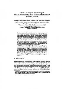
Table 1: Experimental results for n = 10. Interval for b1
b 2 − b1
RSGR OP T
[A/4, A/2) [A/4, A/2) [A/4, A/2) [A/2, 3A/4) [A/2, 3A/4) [A/2, 3A/4) [3A/4, A) [3A/4, A) [3A/4, A)
(0, 10] (10, 100] (100, 1000] (0, 10] (10, 100] [100, 1000] (0, 10] (10, 100] (100, 1000]
1.146215 1.193226 1.223028 1.020548 1.048857 1.090441 1.027801 1.032412 1.056544
max100 i=1
RSGRi OP Ti
1.395317 1.532669 1.586359 1.100006 1.316561 1.474237 1.167420 1.441846 1.631607
RSGR1 OP T
RSGR2 OP T
RSGR3 OP T
1.411498 1.540146 1.626683 1.478944 1.704705 1.975430 1.146719 1.195518 1.283370
1.193111 1.251648 1.290432 1.028092 1.068175 1.131206 1.063409 1.179593 1.434572
1.204305 1.276607 1.327243 1.266856 1.400590 1.576460 1.055392 1.065919 1.107645
t0 = 1 without loss of generality. The growth rates were generated from the interval [0, 1]. We set A = t0
Qn
i=1 (1 + αi ).
The values of b1 were generated from the intervals [A/4, A/2), [A/2, 3A/4) and
[3A/4, A). The values of b2 − b1 were generated from the intervals (0, 10], (10, 100] and (100, 1000]. Therefore, the combination of all the intervals yields 9 different cases. For a given case, 100 instances were generated. For each instance i, it was solved by the RSGR heuristic and the optimal value was calculated. We denote the corresponding values as RSGRi and OP Ti . Furthermore, to verify the performance of the three parallel procedures, we denote RSGRij as the value yielded by the procedure LSGR(Sj ), j = 1, 2, 3. The average ratio P100
P100
RSGRi i=1 OP Ti /100,
the worst ratio max100 i=1
RSGRi OP Ti ,
RSGRj average ratios i=1 RSGRii /100 are reported in Table 1, where j = 1, 2, 3. For simplicity, RSGRj RSGR OP T , and RSGR for j = 1, 2, 3, as the average ratios mentioned in the above.
and the
we denote
Table 1 indicates that algorithm RSGR yields a solution much better than that yielded individually by each procedure. And a solution produced by algorithm RSGR is on average no more than 9.1% worse than an optimal solution except for b1 ∈ [A/4, A/2). Even for b1 ∈ [A/4, A/2), this value increases to 22.4%. In addition, we evaluated the worst-case behavior of the algorithm. The solution delivered by the algorithm is no more than 63.2% worse than an optimal solution. It indicates that the performance of algorithm RSGR is bounded well, and the proposed algorithm is acceptable for the considered NP-hard problem. Table 1 also indicates that the second procedure performs better than the other two procedures except for b1 ∈ [3A/4, A), while the third procedure performs the best for b1 ∈ [3A/4, A). Furthermore, the relative performance of the procedures was evaluated. Nine different tests with 100 randomly generated instances were performed. For each instance i of each test, we denote RSGRijk as the minimum value of the values yielded by the procedures LSGR(Sj ) and LSGR(Sk ),
14
Table 2: Experimental results for n = 10 and n = 20. Interval for
n = 10
b1
b2 − b1
RSGR12
[A/4, A/2) [A/4, A/2) [A/4, A/2) [A/2, 3A/4) [A/2, 3A/4) [A/2, 3A/4) [3A/4, A) [3A/4, A) [3A/4, A)
(0, 10] (10, 100] (100, 1000] (0, 10] (10, 100] (100, 1000] (0, 10] (10, 100] (100, 1000]
1.033579 1.039559 1.043281 1.006282 1.015927 1.030397 1.012609 1.037631 1.078416
RSGR
above, we denote
RSGRjk RSGR
RSGR31
RSGR12 RSGR
RSGR23 RSGR
RSGR31 RSGR
1.001001 1.001407 1.002068 1.000009 1.000173 1.001068 1.000000 1.003526 1.018389
1.049005 1.067329 1.081569 1.236990 1.324239 1.422773 1.025693 1.024513 1.023082
1.016530 1.016701 1.017546 1.000000 1.000059 1.001103 1.003110 1.004436 1.014696
1.000000 1.000000 1.000000 1.000000 1.000000 1.000000 1.000000 1.000000 1.000060
1.185884 1.190629 1.216755 1.503232 1.513900 1.579965 1.126958 1.125144 1.118945
RSGR
j, k = 1, 2, 3, j 6= k. The average ratios
n = 20
RSGR23
P100
RSGR
RSGRijk i=1 RSGRi /100
were calculated. In the same way as
as the average ratios for simplicity, where j = 1, 2, 3; k = 1, 2, 3; j 6= k.
For n = 10 and n = 20, the results are reported in Table 2; for n = 50 and n = 100, the results are listed in Table 3. From the Tables 2 and 3, we can see that the average ratios 12 RSGR23 RSGR31 { RSGR RSGR , RSGR , RSGR },
RSGR23 RSGR
are the best among
and are almost equal to 1 if n ≥ 20 except the underlined result. But
this is not the case if n is small. For n = 10, the average ratios
RSGR23 RSGR
are larger than 1 except the
underlined result. So we can conclude that RSGR can be revised and simplified through deleting the procedure LSGR(S1 ) if n is large enough. Table 3 shows that the parameter b2 − b1 , i.e., the time duration of the non-available period, has no influence on the ratio only except the bold result if n is large enough. The average ratios
RSGR31 RSGR
are much larger than
RSGR12 RSGR
and
RSGR23 RSGR ,
which
also indicates that the second procedure performs better than others on average.
4
Conclusions
In this paper we considered the problem of scheduling deteriorating jobs on a single machine with an availability constraint. We studied the non-resumable case with the objective of minimizing the makespan and total completion time. We showed that both problems are NP-hard in the ordinary sense. For the makespan problem, we presented an optimal approximation algorithm for the on-line case, and a fully polynomial time approximation scheme for the off-line case. For the total completion time problem, we provided a heuristic and evaluated its effectiveness by computational experiments. The computational results show that the heuristics is efficient in obtaining near-optimal solutions. It will be interesting to find out if an approximation algorithm with a constant worst-case ratio
15
Table 3: Experimental results for n = 50 and n = 100. Interval for
n = 50
b1
b2 − b1
RSGR12
[A/4, A/2) [A/4, A/2) [A/4, A/2) [A/2, 3A/4) [A/2, 3A/4) [A/2, 3A/4) [3A/4, A) [3A/4, A) [3A/4, A)
(0, 10] (10, 100] (100, 1000] (0, 10] (10, 100] (100, 1000] (0, 10] (10, 100] (100, 1000]
1.003285 1.003285 1.003285 1.000000 1.000000 1.000000 1.000786 1.000786 1.000787
RSGR
n = 100
RSGR23
RSGR31
RSGR12 RSGR
RSGR23 RSGR
RSGR31 RSGR
1.000000 1.000000 1.000000 1.000000 1.000000 1.000000 1.000000 1.000000 1.000000
1.319414 1.319414 1.319414 2.069904 2.069904 2.069906 1.353337 1.353337 1.353337
1.000751 1.000751 1.000751 1.000000 1.000000 1.000000 1.000474 1.000474 1.000474
1.000000 1.000000 1.000000 1.000000 1.000000 1.000000 1.000000 1.000000 1.000000
1.572155 1.572155 1.572155 2.634543 2.634543 2.634543 1.584777 1.584777 1.584777
RSGR
RSGR
exists for the total completion time problem. Extending our problems to parallel machines or flowshops is also an interesting issue. In addition, it is worth studying the problem with the objective of minimizing other scheduling performance criteria.
References [1] B. Alidaee, N. K. Womer, Scheduling with time dependent processing times: Review and extensions, J. Oper. Res. Soc., 50 (1999) 711-720. [2] L. G. Babat, Linear functions on the n-dimensional unit cube, Doklady Akademiia Nauk SSSR, 221 (1975) 761-762. (Russian) [3] S. Brown, U. Yechiali, Scheduling deteriorating jobs on a single process, Oper. Res., 38 (1990) 495-498. [4] Z. L. Chen, Parallel machine scheduling with time dependent processing times, Discrete Applied Mathematics, 70 (1996) 81-93. [5] T. C. E. Cheng, Q. Ding, B. M. T. Lin, A concise survey of scheduling with time-dependent processing times, European J. Oper. Res., 152 (2004) 1-13. [6] M. R. Garey, D. S. Johnson, Computers and Intractability: A Guide to the Theory of NPCompleteness, Freeman, San Francisco, CA, 1979. [7] G. V. Gens, E. V. Levner, Approximate algorithms for certain universal problems in scheduling theory, Engineering Cybernetics, 6 (1978) 38-43. (Russian)
16
[8] R. L. Graham, E. L. Lawler, J. K. Lenstra, A. H. G. Rinnooy Kan, Optimization and approximation in deterministic sequencing and scheduling: a survey, Annals of Discrete Mathematics, 5 (1979) 287-326. [9] G. H. Graves, C. Y. Lee, Scheduling maintenance and semi-resumable jobs on a single machine, Naval Res. Logist., 46 (1999) 845-863. [10] J. N. D. Gupta, S. K. Gupta, Single facility scheduling with nonlinear processing times, Comput. Industr. Engrg., 14 (1988) 387-393. [11] D. S. Johnson, The NP-complete columns: an ongoing guide, J. Algorithms, 2 (1981) 402. [12] A. S. Kunnathur, S. K. Gupta, Minimizing the makespan with late start penalties added to processing times in a single facility scheduling problem, European J. Oper. Res., 47 (1990) 56-64. [13] C. Y. Lee, Machine scheduling with an availability constraint, J. Global Optimization, 8 (1996) 395-417. [14] C. Y. Lee, L. Lei, M. Pinedo, Current trend in deterministic scheduling, Annals Oper. Res., 70 (1997) 1-42. [15] G. Mosheiov, Scheduling jobs under simple linear deterioration, Comput. Oper. Res., 21 (1994) 653-659. [16] G. Mosheiov, Scheduling jobs with step-deterioration: minimizing makespan on single and multi-machine, Comput. Industr. Engrg., 28 (1995) 869-879. [17] M. Pinedo, Scheduling: theory, algorithms, and systems, Prentice-Hall, Upper Saddle River, NJ, 2002. [18] C. C. Wu, W. C. Lee, Scheduling linear deteriorating jobs to minimize makespan with an availability constraint on a single machine, Inform. Process. Lett., 87 (2003) 89-93.