Scheduling Linearly Deteriorating Jobs on Multiple Machines. Yi-Chih Hsieh. Department of Industrial Engineering. National Yunlin Polytechnic Institute, Huwei, ...
Scheduling Linearly Deteriorating Jobs on Multiple Machines Yi-Chih Hsieh Department of Industrial Engineering National Yunlin Polytechnic Institute, Huwei, Yunlin 632, Taiwan and Dennis L. Bricker Department of Industrial Engineering University of Iowa, Iowa City, IA 52242 (Revised, March 1997)
Abstract This paper investigates the scheduling problems in which the job processing times do not remain constant but are increasing linear functions of their starting times. Two deteriorating scheduling models, Model 1 and Model 2, for multiple machines are considered, with the goal being to minimize the makespan. In this paper, we propose an efficient heuristic for Model 1 and prove that the ratio of the makespan obtained by the heuristic to the optimal makespan is bounded. For model 2, three heuristics, including a probabilistic heuristic, are proposed for minimizing the makespan. Numerical results are provided to show the efficiency of the approaches in this paper.
1. Introduction and Notations 1.1 Introduction The deteriorating job scheduling problem (DJSP) was introduced by Browne and Yechiali [1]. Unlike the typical scheduling problems in which the processing times are independent and constant (Conway et al. [4] and Pinedo [5]), the DJSP is to schedule a set of jobs in which the processing times of the jobs are not constant but increasing over time, i.e., deteriorating. Therefore the processing times are no longer independent. Such problems occur in maintenance scheduling, cleaning assignments, and manufacturing (Mosheiov [2,3]) and other problems where the proverbial "stitch in time saves nine". Such problems also occur when not the job but the machine is deteriorating, so that jobs processed later require a longer processing time. Assume that N jobs must be scheduled on a single machine and that the original processing time is given by pi , i = 1,2,..., N . Browne and Yechiali [1] proposed optimal scheduling policies that minimize the expected makespan in which the actual processing time for job i is pi + α it i , where α i ∈(0,1) is the so-called deterioration rate and ti is the time at which processing of job i begins. Mosheiov [3] investigated the optimal policy which minimizes the total flow time in which the actual processing time for job i is 1 + α it i . Recently, Mosheiov [2] studied other problems in which the actual processing time for job i is given by α i ti , ti > 0 . All the DJSPs which have been reported thus far are for a single machine. It is well known that the multiple machine scheduling problem to minimize the makespan is NP-hard even if there is no deterioration (Pinedo [5]), that is α i = 0 ∀i (in this case the processing time for job i is pi + α it i = pi ). Obviously, therefore, the DJSP is NP-hard. In this paper, we will study the DJSP to minimize the makespan for multiple machines under the assumption of linear deterioration. Two types of linear deterioration, as introduced by Mosheiov [2] and by Browne and Yechiali [1], respectively, are considered. For the first deterioration model, we propose a heuristic algorithm to minimize the makespan, and prove a bound for the heuristic solution. For
1
the second deterioration model, we propose three heuristics, including a probabilistic heuristic, to minimize the makespan. Computational results are provided to demonstrate the performance of these heuristics. 1.2 Notations Before introducing the models, we define the following notations: N
The total number of jobs to be processed.
M
The total number of available machines.
pi
The original processing time for job i , i = 1,2,..., N .
αi
The deterioration rate for job i , i = 1,2,..., N , α i ∈(0,1).
ti
The time at which processing of job i begins, i = 1,2,..., N .
Pi
The actual processing time for job i , i = 1,2,..., N .
I(j ) I
The ordered index set of jobs processed by machine j , j =1,2,..., M . ≡ {I(1), I(2),..., I(M)} , is a partition of the set of jobs {1,2,..., N }, i.e., I(j1 ) ∩ I( j2 ) = ∅ for j1 ≠ j2 and
A Cmax (I)
M
∪ I( j) = {1,2,..., N} . j =1
Family of all partitions I of {1,2,..., N} . Makespan of jobs on all machines using job partition I . Note that pi is a constant, while Pi is a function of t , namely Pi (t) = pi + α it (or α i t ).
2. Model 1 2.1 Assumptions and Heuristic for Model 1 Following the model discussed in Mosheiov [2], the processing time for job i is Pi = α i ti , i.e., at time zero the jobs require no processing time. (Clearly the problem is nontrivial then only if some jobs can be scheduled only after some time t 0 .) While Mosheiov considered the problem of scheduling a single machine, we consider the problem of N jobs to be scheduled
2
on M identical machines. In both cases, the object is to minimize the makespan. Mosheiov has N
showed that, for the case of the single machine, the optimal makespan is given by t 0 ∏ (1+ α i ), i =1
where t 0 > 0 is the time at which processing begins and is obtained by scheduling the jobs in the order of non-decreasing α.. Clearly, then, for the multiple machine case, the makespan on machine j for the sequence of jobs I(j ) is C j (I( j)) = t0
∏ (1+ α ) , i
i∈I( j )
and the makespan for the assignment of jobs I is Cmax (I) = max {C j (I( j))} . 1≤ j ≤ M
The optimal assignment of jobs is I, which yields the minimum makespan, i.e., Cmax ( Iˆ ) = min{Cmax (I)} . I∈A
In the following, we assume, without loss of generality, that t 0 = 1 for this model. Heuristic 1 Step 0: Reorder the jobs such that α 1 ≥ α 2 ≥ ... ≥ α N . Step 1: Set I(j ) ←∅ , j = 1,2,..., M , and i ← 1. Step 2: Set k ← arg min {Cj (I( j))} 1≤ j ≤ M
Step 3:
I(k) ← I(k) ∪ {} i , i ← i + 1.
Step 4: If i < N , go to step 2. Otherwise, stop. This simple algorithm assigns jobs to machines, one at a time, beginning with the job having the highest deterioration rate. Each job is assigned to the machine which has the shortest makespan (for the partial assignment of jobs).
2.2 Error Bounds for Heuristic 1
3
In this section, we will develop bounds for the ratio of the solution obtained by the heuristic algorithm, denoted by I˜ , to the optimal solution, Iˆ . Let Cmin (I) = min {C j (I( j))} denote the minimal makespan among the M machines for 1≤ j ≤M
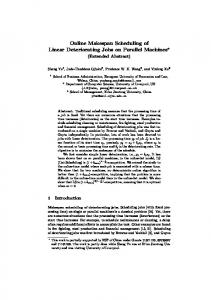
the assignment I . The two quantities, Cmin ( I˜ ) and Cmax ( I˜ ), are illustrated in Figure 1 for M = 3, N = 6. We distinguish between two possible cases for the makespan Cmax ( I˜ ) of the heuristic solution: Case 1: The last job to be assigned, i.e. job N (having the lowest deterioration rate) is assigned to the machine whose makespan determines the overall makespan. For example, this is the case in Figure 1(a) where I˜ = [{1,6},{2,5},{3,4}]. Case 2: The last job to be assigned is assigned to a machine whose makespan does not determine the overall makespan. This is the case in Figure 1(b), for example, where I˜ = [{1}, {2,5}, {3,4,6}].
Cmax ( I˜ )
1 2 3
6
1 2 3
Cmax ( I˜ ) 1 2
5 4
3
Cmin ( I˜ )
1 2 3
5 4
6 Cmin ( I˜ )
(b) Case 2
(a) Case 1
Figure 1. Two cases for six jobs with three machines.
Proposition 1. Let Iˆ denote the optimal assignment, I˜ the assignment obtained by the heuristic algorithm, and I˜ − the assignment of all but the last job (i.e., job N ) by the heuristic algorithm. Then
4
N (a) Cmax ( Iˆ ) ≥ ∏(1+ α i ) i =1
1M
N −1 − ˜ (b) Cmin ( I ) ≤ ∏ (1+ α i ) i =1
, 1M
N Proof. (a) Suppose Cmax ( Iˆ ) < ∏(1+ α i ) i =1 1M
N max Cj ( Iˆ( j)) < ∏ (1 + α i ) 1≤ j ≤M i =1
{
}
M
N
j =1
i =1
. 1M
. By definition, we have
N , which implies that C j ( Iˆ( j)) < ∏ (1 + α i ) i =1
Thus, ∏ C j ( Iˆ( j)) < ∏ (1 + α i ) , which is a contradiction, since N −1 (b) Suppose Cmin ( I˜ − ) > ∏ (1+ α i ) i =1 1M
N−1 min Cj ( I˜ − ( j)) > ∏ (1 + α i ) 1≤ j ≤M i =1
{
}
M
N−1
j =1
i =1
1M
,1 ≤ j ≤ M .
M
N
j =1
i =1
∏ C j ( Iˆ( j)) = ∏(1+ α i ) .
1M
. By definition, we have 1M
N−1 , which implies that C j ( I˜ − ( j)) > ∏ (1 + α i ) i =1
Thus, ∏ C j ( I˜ − ( j)) > ∏ (1 + α i ) , which is a contradiction, since
,1 ≤ j ≤ M .
M
N −1
j =1
i =1
∏ C j ( I˜ − ( j)) = ∏(1+ α i ) .
Lemma 2. If the solution I˜ obtained by Heuristic 1 satisfies case 1, then 1 C max (I˜ ) 1− ≤ (1+ α N ) M . ˆ C max (I ) 1M
N Proof. The optimal assignment satisfies Cmax ( Iˆ ) ≥ ∏(1+ α i ) (because of Proposition 1(a)) i =1 and the heuristic assignment, in case 1, satisfies C ( I˜ ) = C ( I˜ − )(1+ α ) , where I˜ − denotes max
min
N
the assignment of all but the last job (i.e., job N ). Since Cmin ( I˜ − ) ≤ ∏ (1+ α i ) i =1 N −1
1M
Proposition 1(b)), we have 1M
Cmax ( I˜ ) Cmin ( ˜I − )(1 + α N ) ≤ 1M Cmax ( Iˆ ) N (1 + αi ) ∏ i =1
N −1 (1 + αi ) (1+ α N ) ∏ ≤ i=1 N = (1+ α N )1− (1 M ) . 1M (1+ α i ) ∏ i =1
5
(by
Lemma 3. Suppose that the solution I˜ obtained by Heuristic 1 satisfies Case 2, so that the last job to be assigned (job N ) is not the last job to be completed (job x , where 1 < x < N ). Then C max (I˜ ) 1− (1/ M ) −( N − x ) M ≤ ( 1+ α ) 1+ α . ( ) x N C max (Iˆ ) Proof. Denote by I˜ − the partial assignment of the first x − 1 jobs. Since 1M x −1 − − ˜ ˜ ˜ Cmax ( I ) = Cmin ( I )(1+ α x ) and Cmin ( I ) ≤ ∏ (1+ α i ) (the proof is similar to that of i =1 Proposition 1), then 1M
x −1 ( 1+ α ) −1 M ∏ i − N (1+ α x ) Cmax ( I˜ ) Cmin ( ˜I )(1+ α x ) i =1 1− (1 M) ≤ = (1+ α x ) (1 + αi ) 1M ≤ 1M i∏ Cmax ( Iˆ ) N N = x +1 (1+ α i ) (1 + αi ) ∏ ∏ i=1 i =1 ≤ (1+ α x )1− (1 M) (1 + α N )
− (N − x ) M
.
For this case we note that (1 + α x )
1−1 M
≥ (1+ α N )
(N − x ) M
. In addition, Lemma 3
generalizes Lemma 2 if x = N , so that these two lemmas can be reduced to the following theorem.
Theorem 4. Denote by I˜ the solution obtained by Heuristic 1, and by x (1 < x ≤ N ) the index of the last job to be completed, i.e., the job whose completion time is the makespan provided by the heuristic solution I˜ . Denote by Iˆ the optimal solution, which yields the minimum makespan. C ( I˜ ) 1−1 M −( N− x ) M Then max ˆ ≤ (1 + α x ) (1+ α N ) . Cmax ( I ) Note that, as N → ∞ , since N >> M and α x → 0 if α i is uniformly distributed in (0,1), this C ( I˜ ) theorem implies that max ˆ → 1 a.e. as N → ∞ . In other words, Heuristic 1 possesses the Cmax ( I ) asymptotic optimality property.
2.3 Numerical Results for Heuristic 1
6
This section will illustrate some numerical results for Heuristic 1. It should be noted that 1M N ˜ ˆ the bound is an overestimate of the ratio (Cmax ( I ) Cmax ( I ) ), since we have used ∏ (1 + α i ) , i=1 the lower bound of the optimal makespan, rather than the actual optimal makespan, in order to derive the bounds in our proofs. To test this heuristic, we vary the number of jobs, N , from 10 to 500 and vary the number of machines, M , from 2 to 10. The deterioration rates are randomly chosen in the interval (0,1). For each combination of N and M , we generate ten random problems to which we apply Heuristic 1 and compute C ( I˜ ). The average value of the ratios max
Cmax ( I˜ ) 1M
N (1 + αi ) ∏ i=1
for each combination of N and M are summarized in Table 1. From Table 1, one observes that these average ratios (which again are upper bounds on the ratios (C ( I˜ ) C ( Iˆ) ) are all in the interval (1,1.07). It can be found that, in general, when max
max
M is fixed, the bounds on these ratios decrease as the number of jobs increases, while when N is fixed, the bounds on these ratios increase as the number of machines increases. When N =500, the bounds are all in the interval (1,1.006) which illustrates the asymptotic optimality property of Heuristic 1.
7
Table 1. The ratio
Cmax ( I˜ ) 1M
N 1 + α ( ) ∏ i i=1
for I˜ found by Heuristic 1.
Number of jobs
Number of machines
Mean value
10 10 50 50 50 50 50 50 50 50 50 100 100 100 100 100 100 100 100 100 500 500 500 500 500 500 500 500 500
2 3 2 3 4 5 6 7 8 9 10 2 3 4 5 6 7 8 9 10 2 3 4 5 6 7 8 9 10
1.020953 1.067583 1.008652 1.016556 1.026271 1.016038 1.035093 1.042501 1.041331 1.033057 1.057683 1.003722 1.005218 1.008542 1.009012 1.014736 1.021198 1.025501 1.029971 1.033860 1.000868 1.001253 1.001839 1.001273 1.002419 1.002958 1.003344 1.003178 1.005106
8
3. Model 2 3.1 Assumptions and Heuristics for Model 2
As in the model of Browne and Yechiali [1], the actual processing time for job j is now assumed to be Pi (t) = pi + α it , where t is the time at which the processing begins and pi is the original processing time for job i . Unlike Browne and Yechiali, however, we consider multiple machines rather than a single machine. That is, just as was the case of Model 1 in the previous section, we must assign N jobs to M machines. As shown by Browne and Yechiali, for the case of a single machine, the makespan is minimized when the N jobs are scheduled according to increasing values of pi α i , and the optimal makespan is given by M
N
i=1
j =i +1
Cmax ( Iˆ ) = ∑ pi ∏ (1+ α j ). Next we introduce two heuristic algorithms, Heuristic 2 and Heuristic 3, to solve Model 2 of the DJSP with multiple machines. Heuristic 2 Step 0: Reorder the jobs such that
p1 p2 p ≤ ≤ ... ≤ N . α1 α 2 αN
Step 1: Set I(j ) ←∅, j =1,2,..., M, and i ← 1. Step 2: Set k ← arg min {Cj (I)} , where C j (I) = 1≤ j ≤ M
Step 3:
∑
u∈I( j )
pu
∏ (1+ α
v ∈I( j ) & v >u
v
).
I(k) ← I(k) ∪ {} i , i ← i +1
Step 4: If i < N , go to step 2. Otherwise, stop. Heuristic 3 Heuristic 3 differs from Heuristic 2 only in that Step 0 is replaced by Step 0'. 1 − α1 1 − α 2 1− α N Step 0': Reorder the jobs such that ≤ ≤ ... ≤ . p1 p2 pN
9
Heuristic 2 is suggested by the optimal policy for the single machine case, while Heuristic 3 is an adaptation of the LPT (Largest Processing Time first) heuristic rule. That is, if there is no deterioration, i.e., α i = 0 for 1≤ i ≤ N , this heuristic procedure implements the simple LPT rule. We next introduce a variation of the above heuristic approaches which introduces a random element to the order in which the jobs are to be assigned to machines.
Heuristic 4 Heuristic 4 differs from Heuristic 2 in that Step 0 is replaced by the following three steps to order the jobs: Step 0 (1) : X ← {1,2,..., N} , Z(0) ← 0, Z (N + 1) ←1, j ← 1. α α Step 0 (2) : Compute z(i) = i ∑ x , i ∈ X , and Z(i) = ∑ z(j ) . pi x ∈X px j≤ i, j ∈X Generate a random number r ∈(0,1), and let if Z(i − 1) < r ≤ Z(i) and i ∈ X i T[ j] = N if Z(i − 1) < r ≤ Z(i) and i = N + 1 Remove job i from the list X : X ← X \ {i}. Step 0 (3) : j ← j + 1. Return to Step 0 (2) if j < N + 1; else reorder the jobs according toT . This probabilistic ordering is based on the observation that the optimal schedule is often very close to the schedules obtained by Heuristic 2, which will assign a job with a smaller value of the ratio pi α i before those with larger ratios; Heuristic 4 chooses the next job to be assigned with a probability inversely proportional to the ratio pi α i . The algorithm may be reapplied many times, and the minimum of the makespans thus obtained may then be selected as the solution. The results of these three heuristics are shown in the following section.
10
3.2 Numerical Results for Heuristics 2 ,3, and 4
As mentioned before, the DJSP are NP-hard problems, with the number of possible schedules increase drastically with the increase of problem size. Therefore, for most problems of interest, finding the optimal makespan by enumerating all possible schedules explicitly is practically infeasible. We have restricted our test problems in size so as to be able to determine the optimal solutions by enumeration and thereby judge the quality of the heuristic solutions. Although the behaviour of scheduling algorithms on problem instances of small size is a poor guide to their performance on larger problem instances, it is generally true that, as the number of jobs increases, the problem becomes easier in the sense that the ratio of the makespan of a heuristic schedule to the optimal makespan is smaller. For Heuristics 2, 3, and 4, two sets of problems are examined: 10-job problems (shown in Table 2) and 15-job problems (shown in Table 3). The number of machines is fixed at two, the original processing times pi are randomly chosen from a normal distribution with mean 50 and standard deviation 10, and the deterioration rates are randomly generated from a uniform distribution in (0,1). Heuristic 4 is performed 20 times for each 10-job problem, and 45 times for each 15-job problem, and the best schedule is chosen from the solutions generated. The number of jobs was kept relatively small so that the optimal solution (OPT) might be found by a complete enumeration of the possible schedules. From Table 2 and Table 3, one finds that Heuristic 2 performs better than Heuristic 3 for several problems. Comparing the results of Heuristics 2, 3, and 4, we can see in column 8 that the probabilistic algorithm, Heuristic 4, performs quite well, yielding the best solution of the three heuristics for 18 of the 20 problems with ten jobs, and for 16 of the 20 problems with fifteen jobs. In the column headed MIN234/OPT, we observe that the ratio of the best makespan found by the three heuristic algorithms to the optimal makespan are all in the interval (1,1.03) with the average ratios 1.0078 and 1.0075) for 10-job and 15-job cases, respectively, implying that the makespans obtained by the heuristic algorithms are very close to the optimal solutions. 11
Table 2. Comparison of makespan for 10-job 2-machine by using different heuristics.
Prob. No.
OPT
H2
H3
MIN23
1 2 3 4 5 6 7 8 9 10 11 12 13 14 15 16 17 18 19 20
461.33 436.71 647.40 493.85 679.52 489.06 557.22 557.28 381.36 361.00 418.99 502.38 529.73 570.20 609.32 448.42 401.26 408.78 417.84 589.54
461.33 441.47 651.50 498.02 725.84 531.62 589.28 590.05 396.72 382.66 426.83 518.13 551.68 597.79 649.46 457.05 431.02 408.78 427.93 604.15
490.41 441.16 693.33 527.78 722.26 548.27 576.93 593.60 396.78 376.04 431.83 511.33 561.48 615.85 666.04 500.47 418.25 424.85 454.20 642.97
461.33 441.16 651.50 498.02 722.26 531.26 576.93 590.05 396.72 376.04 426.83 511.33 551.68 597.79 649.46 457.05 418.25 408.78 427.93 604.15
H4 468.19 441.16 647.40 493.85 684.93 503.14 562.12 567.45 384.95 361.00 420.90 504.24 529.73 570.20 624.09 448.42 408.07 410.99 422.37 596.28
MIN234 OPT 1.0000 1.0102 1.0000 1.0000 1.0080 1.0288 1.0088 1.0182 1.0094 1.0000 1.0045 1.0037 1.0000 1.0000 1.0243 1.0000 1.0170 1.0000 1.0108 1.0114
Note: OPT = the optimal makespan, H2 = the makespan obtained by Heuristic 2, H3 = the makespan obtained by Heuristic 3, H4 = the best makespan obtained by 20 tries with Heuristic 4, MIN23 = min (H2,H3), MIN234 = min(H2,H3,H4).
12
MIN23 H4 0.9854 1.0000 1.0063 1.0084 1.0545 1.0566 1.0264 1.0398 1.0306 1.0417 1.0141 1.0141 1.0414 1.0484 1.0406 1.0192 1.0250 0.9946 1.0132 1.0132
Table 3. Comparison of makespan for 15-job 2-machine by using different heuristics.
Prob.No. 1 2 3 4 5 6 7 8 9 10 11 12 13 14 15 16 17 18 19 20
OPT 948.46 1048.04 1303.76 1427.64 1043.09 1905.29 1649.09 1021.66 1281.53 1108.31 1068.75 1122.68 1324.16 608.40 1494.89 938.78 659.67 1275.62 1242.80 1162.27
H2
H3
MIN23
965.53 1053.52 1314.35 1453.00 1075.36 2074.13 1714.66 1030.51 1332.24 1144.63 1095.84 1127.06 1387.61 613.54 1506.59 978.62 675.24 1303.94 1286.83 1180.11
1027.20 1146.70 1405.84 1664.80 1102.28 2355.19 1846.54 1158.69 1600.51 1189.29 1093.13 1253.80 1541.63 646.24 1744.69 1178.91 762.81 1590.14 1347.17 1212.81
965.53 1053.52 1314.35 1453.00 1075.36 2074.13 1714.66 1030.51 1332.24 1144.63 1093.13 1127.06 1387.61 613.54 1506.59 978.62 675.24 1303.94 1286.83 1180.11
H4 960.59 1060.99 1330.59 1440.02 1051.06 1935.18 1655.82 1023.05 1298.76 1133.37 1072.94 1142.13 1324.52 608.58 1522.61 947.63 667.32 1275.62 1247.26 1176.25
MIN234 OPT 1.0128 1.0052 1.0081 1.0088 1.0076 1.0157 1.0041 1.0014 1.0134 1.0226 1.0039 1.0039 1.0003 1.0003 1.0078 1.0094 1.0116 1.0000 1.0020 1.0120
Note: OPT = the optimal makespan, H2 = the makespan obtained by Heuristic 2, H3 = the makespan obtained by Heuristic 3, H4 = the best makespan obtained by 45 tries with Heuristic 4, MIN23 = min (H2,H3), MIN234 = min(H2,H3,H4).
13
MIN23 H4 1.0051 0.9930 0.9878 1.0090 1.0231 1.0718 1.0355 1.0073 1.0258 1.0099 1.0188 0.9868 1.0476 1.0081 0.9895 1.0326 1.0119 1.0222 1.0317 1.0033
4. Conclusions In this paper we have studied two models for problems of scheduling deteriorating jobs on multiple machines. For Model 1, in which a job's processing time is proportional to the job’s starting time, we propose a heuristic, prove that the ratio of the makespan obtained by heuristic over the optimal makespan is bounded, and show that our heuristic algorithm possesses an asymptotic optimality property. Numerical results show the effectiveness of this heuristic. For Model 2, in which a job's processing time includes a fixed time in addition to a time proportional to the starting time, we propose three heuristic algorithms. Limited numerical results for problems with two machines and either ten or fifteen jobs, for which we can determine the optimal makespan by a complete enumeration, indicate that these heuristic algorithms provide quite good solutions.
REFERENCES 1. S. Browne and U. Yechiali. Scheduling deteriorating jobs on a single processor. Ops. Res., 38, 495-498 (1990). 2. G. Mosheiov. Scheduling jobs under simple linear deterioration. Comput. Ops. Res., 21, 653-659 (1994). 3. G. Mosheiov. V-shaped policies for scheduling deteriorating jobs. Ops. Res., 39, 979-991 (1991). 4. R. W. Conway, W. L. Maxwell, and L. W. Miller. Theory of Scheduling. Addison-Wesley, Reading, Mass. (1967). 5. M. Pinedo. Scheduling : Theory, Algorithms, and Systems. Prentice-Hall, Englewood Cliffs, NJ. (1995).
14