Scheduling Multiple Continuous Queries to ... - Semantic Scholar

Scheduling Multiple Continuous Queries to Improve QoD∗ Mohamed A. Sharaf, Alexandros Labrinidis, Panos K. Chrysanthis, Kirk Pruhs Department of Computer Science University of Pittsburgh Pittsburgh, PA 15260, USA {msharaf, labrinid, panos, kirk}@cs.pitt.edu

ABSTRACT Quality of Service (QoS) and Quality of Data (QoD) are the two major dimensions for evaluating any query processing system. In the context of the new data stream management stystems (DSMSs), multi-query scheduling has been exploited to improve QoS. In this paper, we are proposing to exploit scheduling to improve QoD. Specifically, we are presenting a new policy for scheduling multiple continuous queries with the objective of maximizing the freshness of the output data streams and hence the QoD of such outputs. The proposed Freshness-Aware Scheduling of Multiple Continuous Queries (FAS-MCQ) policy decides the execution order of continuous queries based on each query’s properties (i.e., cost and selectivity) as well the properties of the input update streams (i.e., variability of updates). Our experimental results have shown that FAS-MCQ can increase freshness by up to 50% compared to existing scheduling policies used in DSMSs.

1.

INTRODUCTION

Data streams processing is an emerging research area that is driven by the growing need for monitoring applications. A monitoring application continuously processes streams of data for interesting, significant, or anomalous events. Monitoring applications have been used in important business and scientific information systems, for example, monitoring network performance, real-time detection of disease outbreaks, tracking the stock market, performing environmental monitoring via sensor networks, providing personalized and customized Web pages. For example, consider the University of Pittsburgh’s Realtime Outbreak of Disease Surveillance System (http://rods.health.pitt.edu). Such a system receives data from different sources (e.g., hospitals, clinics, pharmacies, etc.) and integrates it together in order to detect correlations or abnormal events. In the event of detecting a disease outbreak, CDC and health departments are notified to start mobilizing their resources. ∗This is an extended version of our paper “Freshness-Aware Scheduling of Continuous Queries in the Dynamic Web”, which appears in the Proceedings of the 8th ACM WebDB Workshop (June 2005, held in conjuction with SIGMOD 2005).

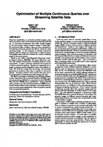
Efficient employment of monitoring applications needs advanced data processing techniques that can support the continuous processing of rapid unbounded data streams. Such techniques go beyond the capabilities of traditional store-then-query Data Base Management Systems. This need has led to a new data processing paradigm and created a new generation of data processing systems, called Data Stream Management Systems (DSMS) that support the execution of continuous queries (CQ) on data streams [23]. Aurora [4], STREAM [18], TelegraphCQ [5], Tribeca [21], Gigascope [10], Niagara [7] and Nile [11] are examples of current prototype DSMSs. In such systems, each monitoring application registers a set of CQs, where a CQ is continuously executed with the arrival of new relevant data (Figure 1). In the Real-time Outbreak of Disease System (RODS) example, the health officials register queries for tracking specific indicators of disease outbreaks. As another example, a user might register a query to monitor news about tsunamis. Thus, as new articles arrive into the system, all the Tsunami-related ones have to be propagated to that user. As such, the arrival of new updates triggers the execution of a set of corresponding queries, since portions of the new updates may be relevant to different queries. The output of such a frequent execution of a continuous query is what we call an output data stream (see Figure 1). In this particular example, an output data stream can be used to continuously update a user’s personalized Web page where a user logs on and monitors updates as they arrive. It can also be used to send email notifications to the user when new results are available. As the amount of updates on the input data streams increases and the number of registered queries becomes large, advanced query processing techniques are needed to efficiently synchronize the results of the continuous queries with the available updates. Efficient scheduling of updates is one such query processing technique which successfully improves the Quality of Data (QoD) provided by interactive systems. In this paper, we are focusing on scheduling continuous queries for improving the QoD of output data streams. QoD can be measured in different ways, one of which is freshness. Freshness, as well as scheduling policies for improving freshness, has been studied in the contexts of replicated databases [8, 9], derived views [13], and distributed caches [19]. To the best of our knowledge, our work is the first to study the problem of freshness in the context of data streams. In this respect, our work can be regarded as complementary to the current work on the processing of continuous queries, which considers only Quality of Service metrics like response time and throughput (e.g., [7, 20, 3, 5, 1]).

Scheduler

1 Input Data Streams

2

3

Continuous Query Q2 1

2

Output Data Stream D2

3

Continuous Query Q1

Output Data Stream D1

Figure 1: A DSMS hosting multiple continuous queries Specifically, the contribution of this paper is proposing a policy for Freshness-Aware Scheduling of Multiple Continuous Queries (FASMCQ). The proposed policy, FAS-MCQ, has the following salient features: 1. It exploits the variability of the processing costs of different continuous queries registered at the DSMS. 2. It utilizes the divergence in the arrival patterns and frequencies of updates streamed from different remote data sources. 3. It considers the impact of selectivity on the freshness of output data stream. To illustrate the last point on the impact of selectivity, let us assume a continuous query which is used to project the number of trades on a certain stock, if its price exceeds $60. Further, assume that there is a 50% chance that this stock’s price exceeds $60. With the arrival of a new update, if the new price is greater than $60 then a new update is added to the continuous output data stream. Otherwise, the update is discarded and nothing is added to the output data stream. So, in this particular example, the arrival of a new update renders the continuous output data stream stale with probability 50%. FAS-MCQ exploits such probability of staleness in order to maximize the overall QoD. Beyond the basic FAS-MCQ policy, we have also explored a weighted version of our FAS-MCQ scheduling policy that supports applications in which queries have different priorities. These priorities could reflect criticality, and hence their importance with respect to QoD captured by freshness, or popularity, and thus be used to optimize the overall user satisfaction. In order to evaluate our proposed scheduling policies, we have implemented a simulator of such DSMS scheduler and ran extensive experiments. As our experimental results have shown, FAS-MCQ can increase freshness by up to 50% compared to existing scheduling policies used in DSMSs. FAS-MCQ achieves this improvement by deciding the execution order of continuous queries based on individual query properties (i.e., cost and selectivity) as well as properties of the update streams (i.e., variability of updates). The rest of this paper is organized as follows. Section 2 provides the system model. In Section 3, we define our freshness-based

QoD metrics. Our proposed policies for improving freshness is presented in Section 4. Section 5 describes our simulation testbed, whereas Section 6 discusses our experiments and results. Section 7 surveys related work. We conclude in Section 8.

2. SYSTEM MODEL We assume a data stream management system (DSMS) where users register multiple continuous queries over multiple input data streams (as shown in Figure 1). Data streams consist of updates at remote data sources that are either continuously pushed to the DSMS or frequently pulled from the data sources. For example, sensor networks readings are continuously pushed to the DSMS, whereas updates to Web databases are frequenly pulled using Web crawlers. Each update ui is associated with a timestamp ti . This timestamp is either assigned by the data source or by the DSMS. In the former case, the timestamp reflects the time when the update took place, whereas in the latter case, it represents the arrival time of the update at the DSMS. In this work, we assume single-stream queries where each query is defined over a single data stream. However, data streams can be shared by multiple queries, in which case each query will operate on its own copy of the data stream. Queries can also be shared among multiple users, in which case the results will be shared among them. Improving the QoD in the context of multi-stream queries as well as shared queries or operators is part of our future work. A single-stream query plan can be conceptualized as a data flow diagram [4, 1] (Figure 1): a sequence of nodes and edges, where the nodes are operators that process data and the edges represent the flow of data from one operator to another. A query Q starts at a leaf node and ends at a root node (Or ). An edge from operator O1 to operator O2 means that the output of operator O1 is an input to operator O2 . Additionally, each operator has its own input queue where data is buffered for processing. As a new update arrives at a query Q, it passes through the sequence of operators of Q. An update is processed until it either produces an output or until it is discarded by some predicate in the query. An update produces an output only when it satisfies all the predicates in the query.

Ideal output data stream

Fresh Stale

Actual output data stream

t1

t2

Tx

t3 Ty

Figure 2: An example on measuring the freshness of a data stream In a query, each operator Ox is associated with two values: • processing time or cost (cx ), and • selectivity or productivity (sx ). Recall that in traditional database systems, an operator with selectivity sx produces sx tuples after processing one tuple for cx time units. sx is typically less than or equal to 1 for operators like filters. Selectivity expresses the behavior or power of a filter. Additionally, for a query Qi , we define three parameters 1. maximum cost (Ci ), 2. total selectivity or total productivity (Si ), and 3. average cost (Ciavg ). Specifically, for a query Qi that is composed of a single stream of operators < O1 , O2 , O3 , ..., Or >, Ci , Si and Ciavg are defined as follows 1 :

Ci = c1 + c2 + ... + cr Si = s1 × s2 × ... × sr Ciavg = c1 + c2 × s1 + c3 × s2 × s1 + ... + cr × sr−1 × ... × s1 The total selectivity measures the probability that a new update will satisfy all the query predicates while the average cost measures the expected time for processing a new update until it produces an output or until it is discarded. The average cost is computed as follows. An update starts going through the chain of operators with O1 , which has a cost of c1 . With a “probability” of s1 (equal to the selectivity of operator O1 ) the update will not be filtered out, and as such continue on to the next operator, O2 , which has a cost of c2 . Moving along, with a “probability” of s2 the update will not be filtered out, and as such continue on to the next operator, O3 , which has a cost of c3 . Up until now, on average, the cost will be C avg = c1 + c2 × s1 + c3 × s2 × s1 . This is generalized in the formula for Ciavg above as in [24]. The maximum cost is a special case of the average cost when the selectivity of each operator in a single-stream query is equal to 1. 1 In the rest of the paper, we use lower-case symbols to refer to operators’ parameters and upper-case ones for queries’ parameters.

3. FRESHNESS OF DATA STREAMS In this section, we describe our proposed metric for measuring the quality of output data streams. Our metric is based on the freshness of data and is similar to the ones previously used in [8, 13, 19, 9, 14]. However, it is adapted to consider the nature of continuous queries and input/output data streams.

3.1 Average Freshness for Single Streams

In a DSMS, the output of each continuous query Q is a data stream D. The arrival of new updates at the input queue of Q might lead to appending a new tuple to D. Specifically, let us assume that at time t the length of D is | Dt | and there is a single update at the input queue; also with timestamp t. Further, assume that Q finishes processing that update at time t
. If the tuple satisfies all the query’s predicates, then | Dt
|=| D | +1, otherwise, | Dt
|=| D |. In the former case, the output data stream D is considered stale during the interval [t, t
] as the new update occurred at time t and it took until time t
to append the update to the output data stream. In the latter case, D is considered fresh during the interval [t, t
] because the arrival of a new update has been discarded by Q. Obviously, if there is no pending update at the input queue of D, then D would also be considered fresh. Formally, to define freshness, we consider each output data stream D as an object and F (D, t) is the freshness of object D at time t which is defined as follows:  1 if ∀u ∈ It , σ(u) is false F (D, t) = (1) 0 if ∃u ∈ It , σ(u) is true where It is the set of input queues in Q at time t and σ(u) is the result of applying Q’s predicates on update u. To measure the freshness of a data stream D over an entire discrete observation period from time Tx to time Ty , we have that: F (D) =

Ty X 1 F (D, t) Ty − Tx t=T

(2)

x

Figure 2 shows an example on measuring the freshness of a data stream. Specifically, the figure shows two output data streams; 1) the ideal stream which shows the times instants when updates became available at the DSMS; and 2) the actual stream which shows the time instants when updates became available to the user. The delay between the time an update is available at the system until the time it is propagated to the user is composed of two intervals: 1) the interval where the continuous query is waiting to be scheduled for execution; and 2) the interval where the continuous

query is processing the update. The sum of these two intervals represents the overall interval when the output data stream deviates from the ideal one. That is, when the output data stream is stale compared to the physical world. In the example illustared in Figure 2, the output data stream is stale for the intervals t1 , t2 and t3 . Hence, the staleness of the data stream is computed as: (t1 + t2 + t3 )/(Ty − Tx ), equivalently, the freshness of the data stream is computed as: ((Ty − Tx ) − (t1 + t2 + t3 ))/(Ty − Tx ).

3.2 Average Freshness for Multiple Streams Having measured the average freshness for single streams, we proceed to compute the average freshness over all the M data streams maintained by the DSMS. If the freshness for each stream, Di , is given by F (Di ) using Equation 2, then the average freshness over all data streams will be: M 1 X F = F (Di ) M i=1

(3)

3.3 Fairness in Freshness Ideally, all data streams in the system should experience perfect freshness. However, this is not always achievable. Especially when the DSMS is loaded, we can have data streams with freshness that is less than perfect, because of a “back-log” of updates that cannot be processed in time [13]. In such a case, it is desirable to maximize the average freshness in addition to minimizing the variance in freshness among different data streams. Minimizing the variance reflects the system’s fairness in handling different continuous queries. In this paper, we are measuring fairness as in [17]. Specifically, we compute the average freshness of each output data stream. Then, we measure fairness as the standard deviation of freshness measured for each data stream. A high value for the standard deviation indicates that some classes of data streams received unfair service compared to others. That is, they were stale for a longer intervals compared to other data streams. A low value for the standard deviation indicates that the difference in service (freshness) among different data streams is negligible, and, as such, the DSMS handled all streams in a fair manner.

4.

FRESHNESS-AWARE SCHEDULING OF MULTIPLE CONTINUOUS QUERIES

In this section we describe our proposed policy for Freshness-Aware Scheduling of Multiple Continuous Queries (FAS-MCQ). Current work on scheduling the execution of multiple continuous queries focuses on QoS metrics [3, 5, 1] and exploits selectivity to improve the provided QoS. Previous work on synchronizing database updates exploited the amount (frequency) of updates to improve the provided QoD [8, 19, 9]. In contrast, our proposal, FAS-MCQ, exploits both selectivity and amount of updates to improve the QoD, i.e., freshness, of output data streams.

4.1 Scheduling without Selectivity

Assume two queries Q1 and Q2 , with output data streams D1 and D2 . Each query is composed of a set of operators, each operator has a certain cost, and the selectivity of each operator is one. Hence, we can calculate for each query Qi its maximum cost Ci as shown in Section 2. Moreover, assume that there are N1 and N2 pending updates for queries Q1 and Q2 respectively. Finally, assume that the current wait time for the update at the head of Q1 ’s queue is

W1 , similarly, the current wait time for the update at the head of Q2 ’s queue is W2 . Next, we compare two policies X and Y . Under policy X, query Q1 is executed before query Q2 , whereas under policy Y , query Q2 is executed before query Q1 . Under policy X, where query Q1 is executed before query Q2 , the total loss in freshness, LX , (i.e., the period of time where Q1 and Q2 are stale) can be computed as follows: LX = LX,1 + LX,2

(4)

where LX,1 and LX,2 are the staleness periods experienced by Q1 and Q2 respectively. Since Q1 will remain stale until all its pending updates are processed, then LX,1 is computed as follows: LX,1 = W1 + (N1 C1 ) where W1 is the current loss in freshness and (N1 × C1 ) is the time required until applying all the pending updates. Similarly, LX,2 is computed as follows: LX,2 = (W2 + N1 C1 ) + (N2 C2 ) where W2 is the current loss in freshness plus the extra amount of time (N1 × C1 ) where Q2 will be waiting for Q1 to finish execution. By substitution in Equation 4, we get LX = W1 + (N1 C1 ) + (W2 + N1 C1 ) + (N2 C2 )

(5)

Similarly, under policy Y in which Q2 is scheduled before Q1 , we have that the total loss in freshness, LY will be: LY = (W1 + N2 C2 ) + (N1 C1 ) + W2 + (N2 C2 )

(6)

In order for LX to be less than LY , the following inequality must be satisfied: N1 C1 < N2 C2

(7)

The left-hand side of Inequality 7 shows the total loss in freshness incurred by Q2 when Q1 is executed first. Similarly, the righthand side shows the total loss in freshness incurred by Q1 when Q2 is executed first. Hence, the inequality implies that between the two queries, we start with the one that has the lower Ni Ci value. Similarly, in the general case, where there are more than 2 queries ready for execution, we start with the one that has the lowest Ni Ci value since it will have the minimum negative impact on the other queries in the system.

4.2 Scheduling with Selectivity Assume the same setting as in the previous section. However, assume that the productivity of each query Qi is Si which is computed as in Section 2. The objective when scheduling with selectivity is the same as before: we want to minimize the total loss in freshness. Recall from Inequality 7 that the objective of minimizing the total loss is equivalent to selecting for execution the query that minimizes the loss in freshness incurred by the other query. In the presence of selectivity, we will apply the same concept.

However, we first need to compute for each output data stream Di its staleness probability (Pi ) given the current status of the input data stream. This is equivalent to computing the probability that at least one of the pending updates will satisfy Qi ’s predicates. Hence, Pi = 1 − (1 − Si )Ni , where (1 − Si )Ni is the probability that all pending updates do not satisfy Qi ’s predicates. Now, if Q2 is executed before Q1 , then the “expected” loss in freshness incurred by Q1 only due to the impact of processing Q2 first is computed as: LQ1 = P1 × N2 × C2avg

(8)

where N2 × C2avg is the expected time that Q1 will be waiting for Q2 to finish execution and P1 is the probability that D1 is stale in the first place. For example, in the extreme case of S1 = 0, if Q2 is executed before Q1 , it will not increase the staleness of D1 since all the updates will not satisfy Q1 . However, at S1 = 1, if Q2 is executed before Q1 , then the staleness of D1 will increase by N2 × C2avg with probability one. Similarly, if Q1 is executed before Q2 , then the expected loss in freshness incurred by Q2 only due to processing Q1 first is computed as:

4.4 Discussion It should be noted that under our policy, the priority of a query increases as the processing of an update advances. For instance, let us assume that a query has just been selected for execution. At that moment, the priority of the query is equal to the priority of its leaf node or leaf operator. After the leaf finishes processing the update, the priority of the next operator, say Ox , is computed as shown earlier. Intuitively, Sx and Cxavg are greater than S and C avg of the leaf operator because the remaining processing cost decreases and the expected productivity might increase too. Additionally, Nx is equal to one and our priority function monotonically increases with the decrease in N . Thus, overall, the priority of Ox is higher than that of the leaf node. Similarly, the priority of each operator in the query is higher than the priority of the operator preceding it. As such, a query Qi is never preempted unless a new update arrives and that new update triggers the execution of a query with a higher priority than Qi . Also note that under our priority function (Equation 11), FAS-MCQ behaves as follows:

(9)

1. If all queries have the same number of pending tuples and the same selectivity, then FAS-MCQ selects for execution the query with the lowest cost.

In order for LQ2 to be less than LQ1 , then the following inequality must be satisfied:

2. If all queries have the same cost and the same selectivity, then FAS-MCQ selects for execution the query with less pending tuples.

LQ2 = P2 × N1 × C1avg

N1 C1avg P1