and the normalized mean field annealing technique, respectively, to resolve a ... THE JOB-SHOP scheduling problem is involved in various applications, such as ...
490
IEEE TRANSACTIONS ON SYSTEMS, MAN, AND CYBERNETICS—PART B: CYBERNETICS, VOL. 29, NO. 4, AUGUST 1999
Scheduling Multiprocessor Job with Resource and Timing Constraints Using Neural Networks Yueh-Min Huang and Ruey-Maw Chen
Abstract— The Hopfield neural network is extensively applied to obtaining an optimal/feasible solution in many different applications such as the traveling salesman problem (TSP), a typical discrete combinatorial problem. Although providing rapid convergence to the solution, TSP frequently converges to a local minimum. Stochastic simulated annealing is a highly effective means of obtaining an optimal solution capable of preventing the local minimum. This important feature is embedded into a Hopfield neural network to derive a new technique, i.e., mean field annealing. This work applies the Hopfield neural network and the normalized mean field annealing technique, respectively, to resolve a multiprocessor problem (known to be a NP-hard problem) with no process migration, constrained times (execution time and deadline) and limited resources. Simulation results demonstrate that the derived energy function works effectively for this class of problems.
I. INTRODUCTION
T
HE JOB-SHOP scheduling problem is involved in various applications, such as communications, industrial control, operations research, and production planning. The concept of scheduling is similar to that of static scheduler in an operating system. Most problems in those applications are NP-complete. This fact implies that an optimal solution for a large scheduling problem is quite time-consuming, as in the traveling salesman problem (TSP). Willems and Rooda translated the job-shop scheduling problem into a format of linear programming and, then, mapped it into an appropriate neural network structure to obtain a solution [1]. Foo and Takefuji employed integer linear programming neural networks to solve the scheduling problem by minimizing the total starting times of all jobs with precedence constraint [2]. Meanwhile, Zhang et al. proposed a neural network method based on linear programming, in which preemptive jobs are scheduled on the basis of their priorities and deadlines [3]. Cardeira and Mammeri investigated the multiprocessor real-time scheduling by applying the -out-ofrule to a neural network [4]. Chang and Jeng employed a nonenergy-based neural network to derive an optimal solution without convergence procedure [5]. The above investigations concentrated on the preemptive jobs (processes) executed on multiple machines (multiprocessor) with job transfer allowed by applying a neural network. Also in [6], Hanada and Ohnishi developed a parallel algorithm based on a neural network for preemptive task scheduling problems by allowing for a Manuscript received April 2, 1997; revised August 30, 1998 and November 8, 1998. This paper was recommended by Associate Editor J. Rozenblit. The authors are with the Department of Engineering Science, National Cheng-Kung University, Tainan 701, Taiwan, R.O.C. Publisher Item Identifier S 1083-4419(99)05271-1.
task transfer among machines. Gallone et al. presented a set of nonpreemptive tasks on a single machine scheduled by applying the -out-of- rule to Hopfield neural network [7]. As generally known, most scheduling problems are combinatorial, thereby ensuring the optimization process by a neural network. More recent investigations have constructed the energy functions for scheduling problems primarily by using either linear programming or the -out-of- rule applied to neural networks. In addition, most scheduling problems are limited to the preemptive and migratory processes on a multiprocessor and, therefore, only consider the timing constraint. In some multiprocessor systems, task scheduling does not include only a timing constraint. For instance, the display system on an advanced avionics system may consist of two or more display processors. Each processor is responsible for different tasks containing the timing constraint without allowing task migration between processors. In addition, tasks utilize shareable resources such as triple channel display component for output display data and cooperative memory component for data exchange. Restated, tasks do not use the same resource simultaneously. To facilitate the pilot’s control action, all tasks must be properly scheduled to provide the pilot with some useful information. Otherwise, a hazardous situation is inevitable. Therefore, this study focuses mainly on resolving the generic problem similar to the above situation. The Hopfield neural network (HNN) [8] proposed by Hopfield and Tank in 1985, which contains a symmetrically interconnected network, provides an effective means of solving combinatorial optimization problems such as the TSP [8], [9]. Basically, HNN is characterized by the rapid minimization of energy functions. The change of neuron state is based on a deterministic rule. That is, the state becomes 1 when the neuron output is positive, 0 when the neuron output is negative; it remains unchanged when the neuron output is zero. Although acceptable results obtained from this method are not guaranteed to be optimum. Among the previous attempts to eliminate this undesirable feature, stochastic simulated annealing (SA) is the most efficient means. Kirkpatrick et al. [10] viewed simulated annealing as a stochastic method for combinatorial optimization problem. Foo and Takefuji [11] later presented a stochastic neural network for solving the jobshop scheduling problem. That investigation applied simulated annealing to obtain an optimal or a near-optimal solution to the job-shop problem. SA involves introducing a synaptic noise (or thermal noise) by thermal fluctuations, subsequently allowing one to prevent the local minimum and to reach
1083–4419/99$10.00 1999 IEEE
Authorized licensed use limited to: National Cheng Kung University. Downloaded on April 26,2010 at 06:23:59 UTC from IEEE Xplore. Restrictions apply.
HUANG AND CHEN: SCHEDULING MULTIPROCESSOR JOB
the global minimum by the equilibrium established through a gradual lowering of the temperature. On the other hand, HNN corresponds to the noiseless system. The neuron state updates are based on the Boltzmann state-transition rule, implying that a state change is acceptable if results in a decrease in energy. Otherwise the Boltzmann probability is used to determine the acceptance. However, HNN is limited by a time-consuming operation, i.e., a slow convergence. The mean field annealing (MFA) [12] algorithm is derived from SA by applying the mean field approximation technique, which contains the merits of SA and HNN. The normalized MFA provides an efficient means of solving combinatorial optimization problems [13], [14], [17], [18]. In light of above developments, this work investigates the job-scheduling problem of a multiprocess on a multiprocessor with the timing as well as resource constraints. An energy function similar to the TSP derived by Hopfield and Tank is also proposed. This energy function actually consists of all constraint items. Our results demonstrate that the energy change is always negative via formal mathematical derivations. Therefore, HNN can be used to obtain the weighting and threshold matrices and, then, proceed with the process to obtain the solution. In addition, the normalized MFA neural network can also obtain the synaptic weights. By doing so, the threshold values and the annealing techniques can be applied to the optimization search. The rest of this paper is organized as follows. Section II describes our scheduling problem and derives the corresponding energy function according to the problem’s intrinsic constraints. Section III briefly reviews the HNN and normalized MFA algorithms and, then, translates the derived energy functions to both algorithms. Section IV provides mathematical proof of the convergence of the energy functions. Next, in Section V, the simulations are presented under two algorithms, HNN and normalized MFA. Discussion and conclusions are finally made in Section VI.
II. ENERGY FUNCTION Our scheduling problem domain considers jobs (or promachines (or processors). Although job-shop cesses) and scheduling problems markedly differ from case to case, the following assumptions are made regarding our problem domain. First, the execution time of each job is predetermined. In addition, although execution time of each job is often difficult to calculate, calculating the machine cycles or some heuristic rules methods can estimate the time. Second, a job can be segmented and the execution of each segment is preemptive. Third, different segments of a job cannot be assigned to different machines, implying that no job migration is allowed between machines. The constraints imposed on proposed model are a deadline for each job and a processing time with limited available resources on the system. Furthermore, a resource instant is not permitted to migrate to any other machine. Above assumptions are quite feasible based on the observation of the display system depicted in the previous section. Based on these assumptions, we attempt to obtain a set of job schedules.
491
Fig. 1. Three-dimensional Hopfield and Tank network.
To resolve this problem, we focus on one of the applications of the neural network, “optimization.” An optimization algorithm attempts to search for states (solution) which satisfy a set of constraints such that a Hopfield objective function (energy/cost function) is maximized or minimized. In this section, we first derive the energy function of the problem in terms of all constraints. Instead of using linear programming or the -out-of- rules to develop the energy function, we directly formulate the cost function according to constraints term by term. Herein, the objective function is constructed from two aspects: the constraint concerned and the design goal proposed. The constraints can be further categorized into two types. The first is the output state constraint for confining the output states to a steady representation; the other is the deadline and resource constraint. Herein, scheduling involves the job, machine, and time variables as depicted in Fig. 1, where the “ ” axis denotes the “job” variable and represents a job with a range from 1 to , the total number of jobs to be scheduled; where the “ ” axis denotes the “machine” variable and any point on the axis represents a dedicated machine identified from 1 to , the total number of machines to be operated; where the “ ” axis denotes the “time” variable and represents a specific time which should be less than or equal is to , the deadline of the job. Thus, a state variable defined as representing whether or not the job is executed on machine at a certain time . In addition, the activated neuron denotes that the job is run on machine at the time ; otherwise, . Notably, each corresponds to a neuron of the neural network. To deal with the output state constraints, since a machine can only execute one job at a certain time , an energy term can be defined as (1)
are as defined above; the where , , , , , , , and same notations are used hereafter. This term has a minimum or equals zero. value of zero, which occurs when If a job is assigned on a dedicated machine, then all of its segments are executed on the same machine as mentioned earlier. In accordance with this constraint, the energy term is defined as follows:
Authorized licensed use limited to: National Cheng Kung University. Downloaded on April 26,2010 at 06:23:59 UTC from IEEE Xplore. Restrictions apply.
(2)
492
IEEE TRANSACTIONS ON SYSTEMS, MAN, AND CYBERNETICS—PART B: CYBERNETICS, VOL. 29, NO. 4, AUGUST 1999
This item also has a minimum value of zero when or is zero, implying that job can only be executed on at any time. machine or machine The third energy term is defined as follows:
observation implies that the energy term becomes zero upon satisfying the resource constraint. Correspondingly, the total energy with all constraints can be induced as (7)
(3) where denotes the processing time required by job , implying that the time spent by all segments of job should be equal . to . Therefore, this term yields zero when In addition, another state constraint energy term is introduced by (4) This term provides a supplemental constraint for (1) to prevent and from becoming zero. By doing so, (1) is both satisfied. Thus, this energy term should also reach a minimum value of zero. Regarding the deadline constraint, no segment of a job can be assigned to a time later than the deadline of the job. Hence, the energy terms are defined as follows: (7) (5)
and if if where represents the deadline of the job and is the Unit step function. This definition obviously reveals that when a segment of a job is assigned later than the deadline , , , this energy term is larger than zero when . The larger the difference implies a larger and energy value. In contrast, this energy term has a value zero as and . long as As for the resource constraint, two jobs are not allowed to use the same resource simultaneously. In addition, the resource is nonpreemptive so that the energy term can be generated as follows: (6)
, , , , , and refer to weighting facwhere tors and are assumed herein to be positive constants in our discussion. Next, consider the second aspect of constructing the objective functions, the design goal consideration. A scheduler generally focuses on arranging a set of jobs in terms of some criteria, such as the shortest time flow (total time consumed), the shortest turnaround time, and the shortest waiting time. This work concentrates mainly on typical scheduling problems with constraint satisfaction, such as the described display system. In the following section, HNN and normalized MFA are used to solve these constraint satisfaction scheduling problems. III. HNN
AND
MFA ALGORITHM
By using the generated energy function described in the previous section, this function is transformed into the corresponding neural network for utilizing the HNN and the normalized MFA algorithm. A. HNN
where denotes the quantity of available resource instances, and are the resource requested matrix elements for jobs, respectively. Where implies that the and indicates that job job requires resource while requests resource . Closely examining this term reveals and that, when two distinct jobs are scheduled (say ) to be executed at the same time on different cannot utilize the same machines and , machines and or is zero because resource at the time , i.e., either each available resource is unique for a dedicated machine. This
The Hopfield neural network has been increasingly applied to solve optimization problems due to its potential capability for parallel implementation. Its algorithm is based on a gradient-type technique. In the theory of dynamic systems, the Lyapunov function [8], [15], or energy function shown in (8), has verified the existence of stable states. This function is used in HNN to guarantee the convergence of the network system
Authorized licensed use limited to: National Cheng Kung University. Downloaded on April 26,2010 at 06:23:59 UTC from IEEE Xplore. Restrictions apply.
(8)
HUANG AND CHEN: SCHEDULING MULTIPROCESSOR JOB
493
where and denote the neuron states, represents the is the threshold value of the neuron. synaptic weight, and The neuron state is in binary value 0 or 1, thereby correlating with the problem requirement. The state change is according to (9) as follows: if net if net
(9)
B. Normalized MFA Algorithm The MFA formulation is a stochastic neural network based on the Boltzmann state-transition rule. This formulation steers the network toward thermal equilibrium. A state change decreasing the energy is accepted. Otherwise, a probabilistic process is used to cope with the state change which causes an increase in energy. In addition, the probabilistic process depends on the temperature and energy difference between two states as
if net denotes the state value for the th iteration. where In sum, the Hopfield algorithm consists of two steps: and threshold 1) define the memory synaptic weights values ; 2) according to (9), start neuron state updating iterations based on the assumed initial value until no state change occurs at any iteration. The first step refers to the storage phase, while the second is the searching process. To adapt it to our problem, the HNN structure must be expanded into a three dimensional state space as shown in Fig. 1. Therefore, (8) and (9) should be modified into (10) and (11)
(10)
The temperature, , is the magnitude of fluctuation; it is a key parameter in controlling the search direction as well as the step size toward the global minimum. In MFA, the mean approximations of state values are used instead of the actual values. Based on the naive mean field [16], an objective function is provided as (13) where th spin; th spin; input; spin interconnection; and are assumed. Since the system is and assumed to be in equilibrium, the average spin value can be calculated by
if net where
if net (11) if net . To map the energy function of the objective problem to the HNN neural network, (7) and (10) are compared to yield the and the threshold as follows: synaptic weight
denotes the average (mean) of at temperature and where the system dynamics of MFA is identical to the motion of the Hopfield network. Related investigations [13], [14], [17], [18] presented a modified MFA algorithm involving the normalization operation to force the 1-outof- constraints to hold. This algorithm implies that those exclusive items can be eliminated from the energy function. This algorithm also assumes that the equilibrium average spin value follows Boltzmann distribution
the normalization operation is as follows: (14)
(12) where if if is the delta function, and .
. where The normalized MFA algorithm can be summarized in the following steps: 1) randomly set the initial average state value and start with the high temperature; 2) proceed with sequential iterations according to (13) and (14); 3) decrease the annealing temperature and repeat step (2) until the convergence is reached.
Authorized licensed use limited to: National Cheng Kung University. Downloaded on April 26,2010 at 06:23:59 UTC from IEEE Xplore. Restrictions apply.
494
IEEE TRANSACTIONS ON SYSTEMS, MAN, AND CYBERNETICS—PART B: CYBERNETICS, VOL. 29, NO. 4, AUGUST 1999
In (13), and are equivalent to the synaptic weight and threshold values on a neural network, respectively. Notably, applying the normalized MFA algorithm to solve scheduling and before calculating problems involves determining can be the cost function of (13). In (7), the item associating eliminated due to the normalization. The normalization ensures that a machine will process a job at any instance. The cost function is then defined as follows:
same active neuron ( , , ) affects only related items during updating in the subsequent iterations. The energy before updating is
(15) Comparing (13) with (15) allows us to determine similarly as in HNN
IV. CONVERGENCE
OF
and
HNN
The defined energy function leads to convergence during the network iteration. Restated, (7) is an appropriate Lyapunov function for the system. Herein, this finding is proven by a formal mathematical approach. Equation (7) consists of two (which can parts, one containing a neuron ( , , ) state be any neuron of a neural network) using resource and the other containing the rest of the neuron states. Thus, refers to a situation in which machine executes job at indicates that time using resource . In contrast, at time nor utilizes job is neither executed on machine resource . Herein, the equation is divided into two parts to observe the change of the energy with respect to the neuron change. Notably, to guarantee convergence to a state minimum, the state of neuron must be updated in a sequential or an asynchronous manner [15], [20]. Thus, the state of the
Authorized licensed use limited to: National Cheng Kung University. Downloaded on April 26,2010 at 06:23:59 UTC from IEEE Xplore. Restrictions apply.
HUANG AND CHEN: SCHEDULING MULTIPROCESSOR JOB
495
(16)
and apply to the indexed where parenthesized item only and indicates that the condition have , after updating, different values. Similarly, the energy, is derived as follows:
(17)
Hence, according to (16) and (17), the changes of the energy can be computed as follows:
Authorized licensed use limited to: National Cheng Kung University. Downloaded on April 26,2010 at 06:23:59 UTC from IEEE Xplore. Restrictions apply.
496
IEEE TRANSACTIONS ON SYSTEMS, MAN, AND CYBERNETICS—PART B: CYBERNETICS, VOL. 29, NO. 4, AUGUST 1999
(19) According to this equation, the change of energy concerns ), where itself with neuron state change ( , , , , , and correspond to the associated items of , , , , , and , respectively. Closely examining (19) again , i.e., when neuron obviously reveals that when 0 or 1 1, the system is in a stable state changes from 0 . situation and the energy difference is zero 1 ( ) A neuron state change from 0 is processing job at time . Hence, implies that machine according to our output state constraint definition, we can is zero infer that (18) According to (18), the total energy difference is involved in ). This the change of a specific neuron state, i.e., ( difference implies that whenever the state changes from 0 1, 1 0, 0 0, or 1 1, the change has different effects on the energy difference. For convenience, the above energy ) is rewritten as (19) difference (
since a machine at a certain time can process one job only. is zero
because no job transfer is allowed.
equals
because the total execution time of job is has the value of
and
.
because a machine is only allowed to execute one job at a time. is zero as long as the time
Authorized licensed use limited to: National Cheng Kung University. Downloaded on April 26,2010 at 06:23:59 UTC from IEEE Xplore. Restrictions apply.
HUANG AND CHEN: SCHEDULING MULTIPROCESSOR JOB
497
is less than the deadline of job . Furthermore, is also zero
TABLE I WEIGHTING FACTOR
OF
HNN
since indicates that resource is used by job , subsequently forcing . Consequently, the energy , difference, becomes one. Finally, is less than zero when the state for the condition in which the neuron state changes from 1 0, . is also zero for the same has a maximum value of reason given above.
TABLE II WEIGHTING FACTOR
OF
MFA
TABLE III RESOURCE REQUESTED MATRIX
or
since a machine can execute one job at most or does nothing at also has a maximum value of a given time. or TABLE IV TIMING CONSTRAINTS MATRIX
and
are positive.
will be
Consequently, the energy difference, , is less than zero when becomes zero. Correspondingly, the proposed the state energy function is a Lyapunov function. V. SIMULATION RESULTS because the total execution time of job is becomes
and
.
because a machine is only allowed to execute one job at a implies that time. In addition a situation in which , and resource is not used by job , which will force becomes zero, then
Two sets of resource and timing constraints and a number of different initial neuron states were applied for the simulations. The constants of the energy function on (7) and (15) are defined in Tables I and II. The initial temperature for MFA was set to ten and then gradually lowered. Two cooling schedules were applied for proposed in a the simulations: one was conventional SA and the other is an asymptotic convergence proposed by Geman and Geamn of [19]. Tables III and IV list the resource and timing constraints, respectively, for cases 1)–3) with different initial state settings. These cases involve four processes (jobs) in two processors (machines) scheduling. In addition, the scheduling problem with five processes and two processors was simulated as well. Tables VIII and IX display the resource and timing constraint matrices used for case 4). In the simulation, the neuron state update was performed sequentially and 200 iterations were evaluated with complete neuron update each time. The simulation results were dis-
Authorized licensed use limited to: National Cheng Kung University. Downloaded on April 26,2010 at 06:23:59 UTC from IEEE Xplore. Restrictions apply.
498
IEEE TRANSACTIONS ON SYSTEMS, MAN, AND CYBERNETICS—PART B: CYBERNETICS, VOL. 29, NO. 4, AUGUST 1999
TABLE V INITIAL STATES SETTING (CASE 1). (i) HOPFIELD AND TANK NEURAL NETWORK. (ii) MEAN FIELD ANNEALING NEURAL NETWORK
Fig. 3. Simulated scheduling results (case 1): (a) Hopfield, (b) MFA with T = T = log(1 + t), and (c) MFA with T = T 3 0:95. Fig. 2. Energy evolution of neural network (case 1): (a) Hopfield, (b) MFA with T = T = log(1 + t), and (c) MFA with T = T 3 0:95.
played by using a Gantt chart to graphically represent the job schedules. In addition, this chart also contained significant portions of the energy curves during neural network evolution (see Figs. 2 and 4). VI. DISCUSSION
AND
CONCLUSIONS
Simulation results indicate that HNN always goes through an oscillation process to the convergence. On the other hand, the normalized MFA proceeds in a smooth and efficient manner to the convergence. The following features of HNN applied to our domain problem are observed. 1) The convergence is initial state dependent, as in cases i, iii, and v of Table VII. These experienced unstable revolutions and no solutions are obtained. Generally, the initial states with a random distribution arrive to a feasible solution (see Tables V and X). 2) The self-feedback and asymmetric structure of HNN produces the oscillatory behavior during the network updating [9], [20]. This fact can be observed from (12) and with the synaptic weight . Consequently, a solution is not guaranteed and leads to an inevitable oscillatory procedure. In [21], Takefuji and Lee proposed a hystersis binary neuron
Fig. 4. Energy evolution of MFA with different initial states for case 2 and cooling schedule T = T 3 0:95.
model to effectively suppress the oscillatory behaviors of neural dynamics for solving combinatorial optimization problems. Moreover, the weighting factor determination is an intrinsic shortcoming of HNN. The simulations also encountered this drawback. According to the simulation results, some significant consequences for normalized MFA can be obtained:
Authorized licensed use limited to: National Cheng Kung University. Downloaded on April 26,2010 at 06:23:59 UTC from IEEE Xplore. Restrictions apply.
HUANG AND CHEN: SCHEDULING MULTIPROCESSOR JOB
499
DIFFERENT INITIAL STATES SETTING (CASE 2)
Fig. 5. Simulated scheduling results of MFA with
T
=
T
TABLE VI MFA WITH
FOR
T
=
T
3 0:95
AND
T
=
T = log(1
+ t)
3 0:95 for case 2.
Fig. 7. Simulated scheduling results of MFA with case 2(ii) and (b) case 2(i) and (iii).
Fig. 6. Energy evolution of MFA with different initial states for case 2 and cooling schedule T = T = log(1 + t).
1) The normalized MFA produces the same scheduling result, regardless of what initial states are assigned as shown in Figs. 3 and 5. Restated, it is state-independent. 2) closely examining the scheduling results in Figs. 5 and 7 reveals that although MFA are conducted with dif-
T
=
T = log(1
+ t): (a)
ferent annealing procedures, they all arrive to identical outcomes eventually, provided that all the initial states have one unique value as in Table VI-2. Otherwise, the random assignment of the initial states obtain different schedules. 3) although the larger the setting values of initial states imply larger initial energy values, those energies (errors) are dramatically decreased to nearly the same value as long as the MFA neural network starts updating and then goes through a similar stochastic process as that in Fig. 6. The energy function proposed herein works efficiently and can be applied to the class of investigated scheduling problems. Among which, processes are independent without communica-
Authorized licensed use limited to: National Cheng Kung University. Downloaded on April 26,2010 at 06:23:59 UTC from IEEE Xplore. Restrictions apply.
500
IEEE TRANSACTIONS ON SYSTEMS, MAN, AND CYBERNETICS—PART B: CYBERNETICS, VOL. 29, NO. 4, AUGUST 1999
TABLE VII DIFFERENT INITIAL STATES SETTING (CASE 3)
FOR
HNN
TABLE VIII RESOURCE CONSTRAINTS
TABLE IX TIMING CONSTRAINTS
tion required or utilizing memory resources to exchange data. It is assumed that each process can work without waiting for external data. However, the required network implementation depends on the intended applications. The normalized MFA algorithm demonstrates an approach to this kind of scheduling is most problem. The annealing schedule of appropriate for most cases (see Figs. 8–12). This work largely focuses on the problem of resource utilization. For practical implementation, the problem can be
extended to involve the temporal relationship on required resources for each job. Restated, each job requires different resources in a specific order. Basically, the entry of resource requirement matrix (Table VIII) should be enumerated instead of using a binary value to indicate a required order. For example, 0 represents a situation in which the resource is not required, where 1 denotes the corresponding resource that is initially required, and 2 represents the resource required secondly and so forth. This assumption implies/suggests that
Authorized licensed use limited to: National Cheng Kung University. Downloaded on April 26,2010 at 06:23:59 UTC from IEEE Xplore. Restrictions apply.
HUANG AND CHEN: SCHEDULING MULTIPROCESSOR JOB
501
TABLE X INITIAL STATES SETTING (CASE 4). (i) HOPFIELD AND TANK NEURAL NETWORK. (ii) MEAN FIELD ANNEALING NEURAL NETWORK
Fig. 8. Hopfield with different initial states for case 3(i), (iii), and (v).
Fig. 10. Simulated scheduling results of HNN: (a) case 3(ii) and (b) case 3(iv).
Fig. 9. Hopfield with different initial states for case 3(ii) and (iv).
value is the sequence number for the resources requested by jobs. Correspondingly, the energy function expressed in this study should be modified by adding new extra energy terms to satisfy this constraint. A notion similar to the priority scheduling constraint may be involved. A future work should more thoroughly address this issue.
Fig. 11. Energy evolution (case 4): (a) Hopfield and (b) MFA with T = T = log(1 + t).
In terms of complexity, the computational time required for and the consuming each neuron is proportional to time of each iteration is equal to the total neuron multiplied by each neuron computation time .
Authorized licensed use limited to: National Cheng Kung University. Downloaded on April 26,2010 at 06:23:59 UTC from IEEE Xplore. Restrictions apply.
502
IEEE TRANSACTIONS ON SYSTEMS, MAN, AND CYBERNETICS—PART B: CYBERNETICS, VOL. 29, NO. 4, AUGUST 1999
Fig. 12. T
=
Simulated scheduling results: (a) Hopfield, (b) MFA with + 0:5t), and (c) MFA with T = T 3 0:95.
Technologies, Factory Automation, 1995, vol. 1, pp. 509–520. [8] J. J. Hopfield and D. W. Tank, “Neural computation of decision in optimization problems,” Biol. Cybern., vol. 52, pp. 141–152, 1985. , “Computing with neural circuits: A model,” Science, vol. 233, [9] pp. 625–633, Aug. 1986. [10] S. Kirkpatrick, C. D. Gelatt, and M. P. Vecchi, “Optimization by simulated annealing,” Science, vol. 220, pp. 671–680, May 1983. [11] Y. P. S. Foo and Y. Takefuji, “Stochastic neural networks for solving job-shop scheduling—Part 1: Problem representation,” in Proc. IEEE ICNN’88, 1988, pp. 275–282. [12] G. Bilbro, R. Mann, T. Miller W. Snyder, D. E. Van den Bout, and M. White, “Mean field annealing and neural networks,” in Advances in Neural Information Processing System. San Mateo, CA: Morgan Kaufmann, 1989, pp. 91–98. [13] D. E. Van den Bout and T. K. Miller, “A traveling salesman objective function that works,” in Proc. IEEE Int. Conf. Neural Networks, 1988, vol. 3, pp. 299–303. [14] C. Peterson and B. Soderberg, “A new method for mapping optimization problems onto neural networks,” Int. J. Neural Syst., vol. 1, pp. 3–22, 1989. [15] J. J. Hopfield “Neurons with graded response have collective computational properties like those of two-state neurons,” in Proc. Nat. Academy Science, vol. 81, pp. 3088–3092, 1984. [16] D. J. Thouless, P. W. Anderson, and R. G. Palmer, “Solution of solvable model of a spin glass,” Phil. Mag., vol. 35, no. 3, pp. 593–601, 1977. [17] D. E. Van den Bout and T. K. Miller, “Graph partitioning using annealed neural networks,” in Proc. IEEE Int. Conf. Neural Networks, 1989, pp. I:521–I:528. [18] , “Improving the performance of Hopfield–Tank neural network through normalization and annealing,” Biol. Cybern., vol. 62, pp. 129–139, 1989. [19] S. Geman and D. Geman, “Stochastic relaxation, Gibbs distributions, and the Bayesian restoration of images,” IEEE Trans. Pattern Anal. Machine Intell., vol. PAMI-6, pp. 721–741, 1984. [20] M. Takeda and J. W. Goodman, “Neural networks for computation: Number representation and programming complexity,” Appl. Opt., vol. 25, pp. 3033–3046, Sept. 1986. [21] Y. Takefuji and K. C. Lee, “An artificial hystersis binary neuron: A model suppressing the oscillatory behaviors of neuron dynamics,” Biol. Cybern., vol. 64, pp. 353–356, 1991.
T = log(1
Consequently, this algorithm results in an complexity. Thus, the complexity does not grow linearly with the problem size. A future work should also focus on how to reduce the complexity in a scheduling problem. REFERENCES [1] T. M. Willems and J. E. Rooda, “Neural networks for job-shop scheduling,” Contr. Eng. Pract., vol. 2, no. 1, pp. 31–39, 1994. [2] Y. P. S. Foo and Y. Takefuji, “Integer linear programming neural networks for job-shop scheduling,” in IEEE Int. Conf. Neural Networks, 1988, vol. 2, pp. 341–348. [3] C.-S. Zhang, P.-F. Yan, and T. Chang, “Solving job-shop scheduling problem with priority using neural network,” in IEEE Int. Conf. Neural Networks, 1991, pp. 1361–1366. [4] C. Cardeira and Z. Mammeri, “Neural networks for multiprocessor realtime scheduling,” in Proc. 6th Euromicro Workshop Real-Time Systems, 1994, pp. 59–64. [5] C. Y. Chang and M. D. Jeng, “Experimental study of a neural model for scheduling job shops,” in IEEE Int. Conf. Systems, Man, Cybernetics, 1995, vol. 1, pp. 536–540. [6] A. Hanada and K. Ohnishi, “Near optimal jobshop scheduling using neural network parallel computing,” in Proc. IECON’93, Int. Conf. Industrial Electronics, Control, Instrumentation, 1993, vol. 1, pp. 315–320. [7] J. M. Gallone, F. Charpillet, and F. Alexandre, “Anytime scheduling with neural networks,” in Proc. 1995 INRIA/IEEE Symp. Emerging
Yueh-Min Huang was born in Taiwan, R.O.C., in 1960. He received the B.S. degree in engineering science from National Cheng-Kung University, Taiwan, in 1982, and the M.S. and Ph.D degrees in electrical engineering from the University of Arizona, Tucson, in 1988 and 1991, respectively. Since 1991, he has been with the Department of Engineering Science, National Cheng-Kung University, Tainan, Taiwan, where he is an Associate Professor. His research interests include distributed multimedia systems, data mining, and real-time systems. Dr. Huang is a Member of IEEE Computer Society, the American Association for Artificial Intelligence, and the Chinese Fuzzy Systems Association. He was a winner of the 1996 Acer Long-Term Award for Best M.S. Thesis Supervision.
Ruey-Maw Chen was born in Taiwan, R.O.C., in 1960. He received the B.S. and M.S. degrees in engineering science from National Cheng Kung University, Taiwan, in 1983 and 1985, respectively. Currently, he is pursuing the Ph.D. degree in the Department of Engineering Science, National Cheng Kung University. From 1985 to 1994, he was a Senior Engineer on Avionics System Design at Chung Shan Institute of Science and Technology (CSIST). Since 1994, he has been on the technical staff at National Chinyi Institute of Technology. His research interests include scheduling, digital image process, and neural network.
Authorized licensed use limited to: National Cheng Kung University. Downloaded on April 26,2010 at 06:23:59 UTC from IEEE Xplore. Restrictions apply.