1 Introduction. A scheduling problem is usually given by a set T of n tasks, with an associated ... In fact, he solves O(logn) linear programs each one with O(n) constraints and ..... W. H. Freemann and Company, San Francisco, CA, (1979). 9.
Scheduling Independent Multiprocessor Tasks
A. K. Amoura1, E. Bampis2, C. Kenyon3, and Y. Manoussakis1 Universit�e Paris Sud, LRI, B^atiment 490, 91405 Orsay Cedex, France 2 Universit�e d'Evry, LaMI, Bvd des Coquibus, 91025 Evry Cedex, France ENS Lyon, LIP, URA CNRS 1398, 46 All�ee d'Italie, 69364 Lyon Cedex 07, France 1
3
Abstract. We study the problem of scheduling a set of n independent multiprocessor tasks with prespeci ed processor allocations on a xed number of processors. We propose a linear time algorithm that nds a schedule of minimum makespan in the preemptive model, and a linear time approximation algorithm that nds a schedule of length within a factor of (1 + �) of optimal in the non-preemptive model.
1 Introduction A scheduling problem is usually given by a set T of n tasks, with an associated partial order which captures data dependencies between tasks, and a set Pm of m target processors. The goal is to assign tasks to processors and time steps so as to minimize an optimality criterion, for instance the makespan, i.e. the maximum completion time Cmax of any task. Depending on the model, tasks can be preempted or not. In the non-preemptive model, a task once started has to be processed (until completion) without interruption. In the preemptive model, each task can be at no cost interrupted at any time and completed later. If there are no precedence constraints, the tasks are said to be independent. In the most classic model, each task is processed by only one processor at a time. However, as a consequence of the development of parallel computers, new theoretical scheduling problems have emerged to model scheduling on parallel architectures. The multiprocessor task system is one such model1 [7]. In this model, a task may need to be processed simultaneously by several processors. In the dedicated variant of this model, each task requires the simultaneous use of a prespeci ed set of processors. Since each processor can process at most one task at a time, tasks that share at least one resource cannot be scheduled at the same time step and are said to be incompatible. Hence, tasks are subject to compatibility constraints. The present paper is concerned with scheduling independent multiprocessor tasks on dedicated processors, in both the preemptive case and the nonpreemptive case, and the goal is to minimize the makespan Cmax . Following the 1
See [6] for some practical justi cations for considering multiprocessor task systems, and a survey on the main results obtained in multiprocessor task scheduling.
notations of [11,20], we will denote the problem by Pm j xj ; pmtnjCmax in the preemptive case, and Pm j xj jCmax in the non-preemptive case. The preemptive problem. In [18], Kubale proved that the preemptive problem
with an unbounded number of processors, P1 j xj ; pmtnjCmax , is strongly NPhard even when j xj j = 2, (i.e. when each task requires the simultaneous use of at most 2 processors). He used a reduction from the edge multi-coloring problem. However, he also showed that the preemptive problem with a xed number m of processors, Pm j xj ; pmtnjCmax, can be solved by linear programming under the restriction that j xj j = 2. On the other hand, Bianco et al. showed that if m is at most 4, then the preemptive problem Pm j xj ; pmtnjCmax can be solved in linear time [1]. Recently, Kramer [16] showed that Pm j xj ; pmtn; rj jLmax , which is a generalization of Pm j xj ; pmtnjCmax , can be solved by linear programming. In fact, he solves O(logn) linear programs each one with O(n) constraints and O(nm+1 ) variables. In this paper, we also use a linear programming formulation to solve the preemptive problem with a xed number m processors Pm j xj ; pmtnjCmax , in linear time, thereby improving the results of [16,18,1]. Our linear program is inspired from Kenyon and Remila's approximation scheme for strip-packing [14]. The non-preemptive problem. The non-preemptive three-processor problem, i.e.
P3j xj jCmax, has been extensively studied. In [2,13], it is proved to be strongly NP-hard by a reduction from 3-partition. The best approximation algorithm is due to Goemans [9] who proposed a 67 -algorithm improving the previous best performance guarantee of 45 [5]. For unit execution time tasks, i.e. Pm j xj ; pj = 1jCmax, the problem is solvable in polynomial time through an integer programming formulation with a xed number of variables [13]. However, if the number of processors is part of the problem, i.e. P j xj ; pj = 1jCmax, the problem becomes NP-hard. Furhermore, Hoogeveen et al. [13] showed that, for P j xj ; pj = 1jCmax, there exists no polynomial approximation algorithm with performance ratio smaller than 4=3, unless P = NP. In this paper, we use the linear programming formulation of the preemptive problem to get a polynomial time approximation scheme for the non-preemptive problem Pm j xj jCmax for xed m. The rough idea is that it does not matter much whether short tasks are preemptable or not; hence the tasks are separated into long tasks and short tasks, and long tasks are dealt with separately by trying essentially every possible arrangement. This is similar in spirit to Hall and Shmoys' polynomial time approximation scheme for single-machine scheduling [12]. Note that the running time, although linear in terms of n, is super-exponential in terms of 1=�.
2 The algorithm in the preemptive model Given any schedule of the tasks, if we take a snapshot at instant t, we see a certain set of tasks, which are all being processed at t. Thus we are led to
consider con gurations, which correspond to collections of tasks which can be processed simultaneously. With a linear programming approach, our algorithm nds partial schedules associated to the con gurations. A global schedule is then produced by simply merging the obtained partial schedules. We rst need a few de nitions. The type of a task is its associated set of required processors, which is a non-empty subset of f1; 2; : : : ; mg. In general, a type � is just a subset of f1; 2; : : : ; mg. We say that types � and � 0 are compatible if � \ � 0 = ;. We de ne a con guration to be a maximum set of compatible task types. I.e., a con guration is a collection C of non-empty types �i � f1; : : : ; mg such that: 1. 8S�i ; �j 2 C ; �i \ �j = ;, i.e. types of C are pairwise compatible. 2. �i 2C �i = f1; : : : ; mg, i.e. C is maximum. Let #C denote the total number of con gurations, determined by the number m of processors. Given: A xed number m of processors. Input: A set T of n multiprocessor dedicated preemptive tasks. Each task i is de ned by its type and its processing time di . Output: An optimal schedule. The algorithm is in three stages: 1. [Set up the Linear Program]. We partition the tasks of T, according to their types, into subsets T � = fi 2 T j task i has type � g; S one for each possible task type. (We have T = � �f1;::: ;mg T � .) We de ne D� as the total processing time of all the tasks of type �, i.e. X D� = di : i2T �
Let us assign a variable xi to each con guration Ci, whose interpretation will be the length of the time interval during which, if we take a snapshot of the schedule during that interval, the types that we see form con guration Ci . The problem can now be formulated by the following linear program. minimize
#C X
i=1
xi
subject to: 8� � f1; : : : ; mg :
(1)
X i s.t. � 2Ci
xi � D �
(2)
The optimization criterion (1) means that the makespan must have minimum length subject to constraints (2) which guarantee that all the tasks are completed.
2. [Solve the Linear Program]. Let (x�1 ; x�2 ; : : : ; x�#C ) denote the solution to the linear program. 3. [Deducing a preemptive schedule]. A feasible optimal schedule can be constructed in a greedy way as follows. For each type �, at any stage of the construction, some tasks of T � have already been completely scheduled, one task of T � may have been partially scheduled and preempted before completion, and the remaining tasks of T � have not yet been scheduled at all. Take the con gurations Ci such that x�i 6= 0, in some arbitrary order. For each such con guration Ci , we construct a partial schedule of length x�i as follows. Consider all the types � 2 Ci. For every such type �, select rst the partially scheduled task of T � (if there is one), then the remaining tasks of T � in arbitrary order, until the total processing time of the selected tasks becomes greater than or equal to x�i (or until all tasks of T � have been scheduled). If the total processing time is strictly greater than x�i , then the last selected task is preempted so that the total processing time is exactly x�i .
3 Analysis of the preemptive algorithm Lemma 1. The number of con gurations is equal to B(m), the mth Bell number. Proof. The number of con gurations C having k elements, 1 � k � m, is equal to the number of ways to partition a set of m elements into k nonempty disjoint subsets. But this is exactly the Stirling number of the second kind S(m; k) = fkm g [15]. the number of all possible con gurations is given by B(m) = Pm Therefore, th k=1 S(m; k) (which corresponds to the m Bell (or exponential) number [10]). ut Remark 2. Using the fact that S(m; k) = kS(m ? 1; k) + S(m ? 1; k ? 1) (see [15] p.73) we get the crude upper bound B(m) � m!, hence the number of con gurations is a constant (as the number of processors m is xed) independent of the number n of tasks.
Theorem 3. Pmj xj ; pmtnjCmax can be solved in time O(n). Proof. Correctness.
From the de nition of a con guration, we see that within the same con guration tasks with di�erent types are compatible and thus can be scheduled in parallel while tasks with the same type have to be scheduled consecutively. Hence, the obtained schedule is feasible. Furthermore, since tasks can P be preempted, it is obvious that the above linear program gives the length #i=1C x�i of the optimal schedule. Running time.
Step 1: The list of tasks is scanned once, and so this step takes time O(n). Step 2: Since there are (2m ? 1) types of tasks and B(m) con gurations, the
linear program has (2m ? 1) constraints and B(m) variables. Both values are constants and so the linear program can be solved in time O(1). Step 3: Each list T � is scanned once, and so this step takes time O(n). Overall the algorithm runs in time O(n). ut
4 The algorithm in the non-preemptive model We say that a task is preemptable if it can be at no cost interrupted at any time and completed later. We will be led to consider mixed models where some tasks are preemptable and others not. A simple approach to obtain a feasible non-preemptive schedule from a preemptive schedule S is to remove the preempted tasks from S and process them sequentially in a na�ve way at the end of S. The produced schedule has a makespan equal to the makespan of S plus the total processing time of the delayed tasks. However, even if S is optimal preemptive, the schedule thus produced is almost certainly not close to optimal, since there can be a large number of possibly long preempted tasks. Our algorithm does use a preemptive schedule to construct a non-preemptive schedule in the way just described. However, to ensure that the non preemptive solution is close to optimal, only \short" tasks are allowed to be preempted. The intuitive idea of the algorithm is the following: rst, partition the set of tasks into \long" tasks and \short" tasks. For each possible schedule of the long tasks, complete it into a schedule of T, assuming that the short tasks are preemptable. From each such preemptive schedule construct a non-preemptive schedule. Finally, among all the schedules thus generated, choose the one that has the minimum makespan. In what follows, for simplicity we give the algorithm for the three-processor case. Our approach can be directly generalized to deal with the m-processor case for any constant m. We rst need a few de nitions. Given a set of tasks L, a snapshot of L is a set of compatible tasks of L. A relative schedule of L is a sequence of snapshots of L such that each task occurs in a subsequence of consecutive snapshots, and consecutive snapshots are di�erent. Roughly speaking, each relative schedule corresponds to an order of processing of the long tasks. Note that to any given non-preemptive schedule of L, one can associate a relative schedule in a natural way by looking at the schedule at every instant where a task of L starts or ends, and writing the set of tasks of L being processed right after that transition. Also note that the last snapshot is then the empty set. Recall that in section 2, we de ned types and con gurations. We now also need to de ne �-con gurations. Given a type �, a �-con guration is a collection of types �i � � such that: 1. 8S�i ; �j 2 C� ; �i \ �j = �, i.e. types of C� are pairwise compatible. 2. �i 2C �i = �.
Let #C� denote the number of �-con gurations. P Let D denotes the total processing time of all the tasks, i.e. D = ni=1 di. The algorithm is in six stages.
Given: Three processors. Input: A set T of n multiprocessor dedicated non-preemptive tasks, each task
i being de ned by its type and its processing time di ; and a constant � such that 0 < � < 1. opt , where C opt is the Output: A schedule with makespan Cmax � (1 + �)Cmax max optimal makespan. 1. [Partition tasks according to lengths]. Sort the 71=� longest tasks, of lengths d1 � : : : � d71=� . Find i � 1=� such that d7i + : : : + d7i+1 ?1 < �. Let k = 7i. Perform the partition T = T 0 [ L where L is the set of tasks with the k longest execution times. 2. [Construct the relative schedules]. List all possible relative schedules M = (M(0); M(2); : : : ; M(f ? 1)) of L. 3. [Set up linear programs.] During this stage of the algorithm, we assume that the tasks of T 0 are preemptive. For each relative schedule M of L, we determine an optimal schedule for the tasks of T such that the associated relative schedule is M; this is done using the following linear program. Variables. There are three types of variables. First, there is one variable ti for each snapshot of M; it represents the instant in the schedule corresponding to the snapshot M(i). Thus tf ?1 represents the time at which the last task of L terminates its execution. In addition, a variable tf represents the time at which the last task of T terminates its execution. Second, there is one variable e� for each type �, such that e� represents the total time during which the processors of f1; 2; 3g n � are processing tasks of L and the processors of � are not processing tasks of L, i.e. processors of � are either processing tasks of T 0 or idle. Third, for each type � and each �-con guration Ci (�), we de ne a variable xi (�). These variables play the same role as the variables xi of section 2, i.e. they help determine the schedule during the e� amount of time during which the processors of � are available to process tasks of T 0 . Constraints. The constraints are the following: (a)
(
for every i 2 f1; : : : ; f g : ti > ti?1; if tj = nish time of task r started at ti , then tj ? ti = dr
(3)
These constraints mean that the ti's, together with M, de ne a feasible schedule of L2 . 2
Note that there are many more ti 's than equality constraints in general.
(b) The variables e� , � � f1; 2; 3g, are determined from the ti's by linear equations3.
8� e� =
X
i s.t. fprocessors used by M (i)g=f1;2;3gn�
ti+1 ? ti :
(4)
(c) The total lengths of the �-con gurations must t in the corresponding amount of available time e� . For every variable e� , we must have one constraint.
8�
X
Ci (� )
xi (�) � e�
(5)
(d) We must guarantee that we have enough time for the execution of all the tasks of T 0, i.e., for each � 0 � f1; 2; 3g, we put in the constraint
8� 0
X
X
� �� i s.t. � 2Ci (� ) 0
xi (�) � D� ; 0
(6)
0
where D� is the total processing time of all the tasks of T 0 of type � 0 . The linear program's objective is to minimize tf . 4. [Solve the linear programs]. For each relative schedule M, we solve the associated linear program, hence a schedule Schedule(M). 5. [Deducing a non-preemptive schedule]. We now no longer assume that the tasks of T 0 are preemptive. To construct a non-preemptive schedule, we proceed as follows: for each relative schedule M, we consider the set of tasks of T 0 which are preempted in Schedule(M). We modify Schedule(M) by executing these tasks at the end of the schedule in a sequential manner. 6. [Compare all schedules]. Among all the schedules produced in stage 5, output the one that has the smallest makespan. 0
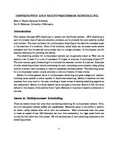
5 Example for the non-preemptive case Consider the task system T given in Table 1. We have D = 90. Assume in addition that k (used in step 1 of the algorithm) is equal to 3. Hence, L = f1; 2; 3g and T 0 = f4; 5; 6; 7;8;9g. A possible relative schedule of the tasks of L is given by the sequence of snapshots M = (f3; 1; 2g; f1;2g; f1g; �) (see Fig. 1 (a)). We shall now construct the linear program corresponding to M. There are ve variables t0, t1 , t2 , t3 and t4 . Let � = 1; � 0 = 13 and � 00 = 123 denote the various sets of processors available at the various times to execute tasks of T 0 . Variable e1 corresponds to the time steps where processors 2 and 3 are processing some tasks of L while processor 1 remains idle or processes some tasks of T 0. We de ne, using similar arguments to those of e1 , variables e13 and e123 3
Thus the variables e� are not really necessary - they can be viewed as a convenient notation.
Table 1. The task system Task name 1 2 3 4 5 6 7 Processing time 25 24 20 6 5 4 3 Required processors 2 3 1 2,3 1,3 1,2 3
3
3
9
8 2 2
9 1 1
5
5 6
1
8
1 4
2
2 e
t0
e
1
t1
13
t2
t3
e
5
5
7 39
123
t4
(b)
(a)
Fig.1. (a) A relative schedule of the long tasks (b) A preemptive schedule respecting the relative schedule of (a).
(the other variables e�i are all 0). Considering all possible partitions of �, � 0 and � 00 , we have the variables x1(�), x1;3(� 0), x13(� 0 ), x1;2;3(� 00 ), x12;3(� 00 ), x1;23(� 00 ), x2;13(� 00 ), x123(� 00). The outline of the linear program is as follows. minimize t4 s.t. t0 = 0;
t1 ? t0 = 20;
t2 ? t0 = 24;
t3 ? t0 = 25
e1 = t 2 ? t 1 = 4 e13 = t3 ? t2 = 1 e123 = t4 ? t3 x1(�) � e1 x1;3(� 0) + x13(� 0 ) � e13 x1;2;3(� 00) + x12;3(� 00 ) + x1;23(� 00 ) + x2;13(� 00) + x123(� 00 ) � e123 x1(�) + x1;3(� 0) + x1;2;3(� 00 ) + x1;23(� 00 ) � D1 = d9 = 1 x1;3(� 0) + x1;2;3(� 00) + x12;3(� 00 ) � D3 = d7 = 3 x1;2;3(� 00) + x2;13(� 00 ) � D2 = d8 = 2 x13(� 0) + x2;13(� 00 ) � D13 = d5 = 5 x1;23(� 00) � D23 = d4 = 6 x12;3(� 00) � D12 = d6 = 4
Note that in this particular case the values of the variables t1 , t2 and t3 are xed since tasks 1, 2 and 3 start at the same time as implied by the rst snapshot f3; 1; 2g of M (this is not true in general). Figure 1 (b) represents the preemptive schedule given by the linear program in the stage 4 of the algorithm, and Fig.2 (a) gives the corresponding non preemptive schedule produced in stage 5. The optimal schedule is given in Fig.2 (b).
9
3
5
3
6 1
5
8
1
8
4 2
4 7
5
2
5
40
(a)
9
6
7 38
(b)
Fig.2. (a) A non-preemptive schedule given by the algorithm respecting the relative schedule of Fig.1.a (b) An optimal schedule.
6 Analysis of the non-preemptive algorithm 6.1 Running time Lemma 4. The total number of relative schedules is at most (k3 )2k . Proof. We create a new snapshot each time there is a new con guration with respect to L, i.e. when a task of L starts or ends its execution. Given that jLj = k, there are at most 2k such events and thus, the sequence contains at most 2k snapshots. Each snapshot consists of at most three tasks chosen among k possibilities, so there are at most k3 possible snapshots. Consequently, there is a constant number, i.e. at most (k3)2k , of relative schedules for the tasks of L. ut Lemma 5. The number of variables of the linear program in stage 3 is O(k). Proof. There are as many variables ti as the number of snapshots of the considered relative schedule M, plus one. Hence, at most 2k + 1 variables. In addition, there is one variable e� for each subset � � f1; 2; 3g, i.e. O(1) variables. Finally, there is one variable of the third type, xi (�), for each �-con guration, where � � f1; 2; 3g, hence O(1) variables. The claim follows. ut
Lemma 6. The number of constraints in the linear program of stage 3 is at most O(k).
Proof. There are at most as many equality constraints of type (3) as long tasks, i.e. k. Inequality constraints of type (3) are as many as variables ti minus one, i.e. at most 2k. There are only O(1) other constraints. ut Proposition 7. The algorithm presented in Section 4 has running time O(n). Proof. A preprocessing phase is needed in order to determine the values of the
total processing times of short tasks for each type �, used in constraints (6). This phase must scan the list of tasks and thus takes O(n) time. Then, it is su�cient to consider for each possible relative schedule the solution of the above linear program, and to choose the relative schedule that gives the schedule of minimum length. Given that the number of possible relative schedules is constant and the solution of the above linear program can be found in O(1) time by the result of Lenstra [19], the result follows. ut
6.2 Correctness
First of all notice that given a relative schedule M of the long tasks, the linear program of stage 3 of the algorithm gives the optimal schedule that respects M and where only short tasks are preemptable. Since at stage 3 of the algorithm all the possible relative schedules of the long tasks are considered, the following result is proved.
Lemma 8. Under the assumption that only short tasks are preemptable, the schedule with the minimum length obtained in stage 4 of the algorithm is optimal. ut
Thus the makespan of the best schedule obtained in stage 4 is a lower bound to the optimal solution of the non-preemptive problem. Now in order to show that the solution provided by the algorithm is close to the optimal schedule, let us assume that the sum D of the execution times of tasks equals 1. This assumption has no e�ect on the result since the problem is invariant by time scaling. In fact, given any we can multiply all the execution P problem instancea T, new instance Ts , solve the problem times by a factor of 1= i2T di to create P on Ts , and then scale the schedule by i2T di to get a schedule of T. The main delay is due to stage 5 of the algorithm. We assume that the execution times are sorted: d0 � d2 � : : : � dn?1. Recall that L is the set of the k longest tasks. The relative schedule (number of snapshots) has length at most 2k, hence at most m(2k) = 6k tasks of T 0 are preempted in the schedule of stage 4 and thus delayed to the end in stage 5. The delay thus incurred is at most dk + : : : + d7k?1. Choice of parameter k. we choose k so that dk +: : :+d7k?1 < �. This is possible
while keeping k = O(c1=�) = O(1) as the following lemma shows. Lemma P 9. Let 1 � d0 � d1 � : : : � dn?1 � 0 be a sequence of numbers such that i di = 1, and let � > 0. Then there exists k � 71=� such that dk + dk+1 + : : : + d7k?1 < �.
Proof. Decompose d0 +: : :+dn?1 into blocks: B0 = d0 +: : :+d6 , B1 = d7 +: : :+
d72?1, : : :, Bi = d7i +: : :+d7i+1 ?1 . Since the sum of all blocks equals 1, at most 1=� of them are greater than �. Take the rst block Bi which is less than �. We have: i � 1=� and for k = 7i , Bi = dk + : : : + d7k?1 < �, hence the lemma. ut Remark 10. If n < 71=� then all the tasks may go into L and the algorithm nds
the optimal solution in constant time.
All we have to do now is apply the algorithm setting jLj = k � 71=�, and we obtain a schedule of length at most (1 + �) times the optimal length. Theorem 11. There is an algorithm A which given a set T of n independent multiprocessor tasks, a xed number m of dedicated processors and a constant � > 0, produces, in time at most O(n), a schedule of T whose makespan is at opt . most (1 + �)Cmax
7 Remarks In this paper we proposed an optimal algorithm for scheduling n preemptable dedicated independent multiprocessor tasks on a xed number of processors, and a polynomial time approximation scheme for the same problem when the tasks are non-preemptable. The approximation algorithm given is polynomial in the size of the problem but super-exponential in 1=�. This result is the best performance guarantee one might hope for since no fully polynomial approximation scheme can be expected as the problem is strongly NP-hard [8]. Of course, it remains interesting to see whether there exists polynomial approximation schemes with lower time complexity in the number of processors m. Note that we conjecture that our algorithm can be extended for the parallel variant of the model (non-dedicated case) as well (see [3] for related work). Some natural questions arise. Do the linear programming ideas developed in this paper have applications to other variants of scheduling?
References 1. L. Bianco, J. Blazewicz, P. Dell'Olmo, and M. Drozdowski. Scheduling Preemptive Multiprocessor Tasks on Dedicated Processors. Performance Evaluation, 20:361371, (1994) 2. J. Blazewicz, P. Dell'Olmo, M. Drozdowski, and M.G. Speranza. Scheduling Multiprocessor Tasks on Three Dedicated Processors. Information Processing Letters, 41:275-280, (1992) 3. J. Blazewicz, M. Drabowski, and J. W�eglarz. Scheduling multiprocessor tasks to minimize schedule length. IEEE Transactions on Computing, 35(5):389-393, (1986) 4. E. G. Co�man, M. R. Garey, D. S. Johnson, and A. S. Lapaugh. Scheduling le transfers. SIAM J. Compt., 14(3):744-780, (1985) 5. P. Dell'Olmo, M. G. Speranza, and Z. Tuza. E�ciency and E�ectiveness of Normal Schedules on Three Dedicated Processors. Submitted.
6. M. Drozdowski. Scheduling Multiprocessor Tasks - An Overview. Private communication, (1996) 7. J. Du, and J. Y-T. Leung. Complexity of Scheduling Parallel Task Systems. SIAM J. Discrete Math., 2(4):473-487, (1989) 8. M. Garey, D. Johnson. Computers and Intractability, A Guide to the theory of NP-completeness. W. H. Freemann and Company, San Francisco, CA, (1979) 9. M. X. Goemans. An Approximation Algorithm for Scheduling on Three Dedicated Processors. Disc. App. Math., 61:49-59, (1995) 10. R. L. Graham, D. E. Knuth, and O. Patashnik. Concrete Mathematics. AddisonWesley, Reading, MA, (1990) 11. R. L. Graham, E. L. Lawler, J. K. Lenstra, and A. H. G. Rinnoy Kan. Optimization and Approximation in Deterministic Sequencing and Scheduling: A Survey. Ann. Disc. Math., 5:287-326, (1979) 12. L.A. Hall and D.B. Shmoys. Jackson's rule for single-machine scheduling: making a good heuristic better. Mathematics of Operations Research, 17:22-35, (1992) 13. J. Hoogeveen, S. L. van de Velde, and B. Veltman. Complexity of Scheduling Multiprocessor Tasks with Prespeci ed Processors Allocation. Disc. App. Math., 55:259272, (1994) 14. C. Kenyon, E. R�emila. Approximate Strip-Packing. Proceedings of the 37th Symposium on Foundations of Computer Science (FOCS), 31-36, (1996) 15. D. E. Knuth. The Art of Computer Programming, Vol.1: Fundamental Algorithms. Addison-Wesley, Reading, MA, (1968) 16. A. Kramer. Scheduling Multiprocessor Tasks on Dedicated Processors. PhD Thesis, Fachbereich Mathematik/Informatik, Universitat Osnabruck, (1995) 17. H. Krawczyk, and M. Kubale. An approximation algorithm for diagnostic test scheduling in multicomputer systems. IEEE Trans. Comput., C-34(9):869-872, (1985) 18. M. Kubale. Preemptive Scheduling of Two-Processor Tasks on Dedicated Processors (in polish). Zeszyty Naukowe Politechniki S�l�askiej, Seria: Automatyka z.100, 1082:145-153, (1990) 19. H.W. Lenstra Integer Programming with a Fixed Number of Variables. Math. Oper. Res., 8:538-548, (1983) 20. B. Veltman, B. J. Lageweg, and J. K. Lenstra. Multiprocessor Scheduling with Communication Delays. Parallel Computing, 16:173-182, (1990)