Scheduling of Iterative Algorithms on FPGA with Pipelined Arithmetic Unit ˇucha1 , Zdenˇek Pohl2 and Zdenˇek Hanz´alek1 Pˇremysl S˚ 1
2
Department of Control Engineering, Faculty of Electrical Engineering Czech Technical University in Prague {suchap,hanzalek}@fel.cvut.cz
Department of Signal Processing, Institute of Information Theory and Automation
[email protected]
Abstract
the loop implies that each operation of the loop is mapped on a hardware unit at a given time, therefore the scheduling theory can be used to find start times of these operations. Cyclic scheduling deals with a set of operations (generic tasks) that have to be performed infinitely often [9]. This approach is also applicable if the number of loop repetitions is large enough. A schedule is called nonoverlapped if all operations belonging to one iteration have to finish before the next operations of the next iteration can start. If operations belonging to different iterations can execute simultaneously, the schedule is called overlapped [17]. An overlapped schedule can be more effective especially if hardware units are pipelined. The periodic schedule is a schedule of one iteration that is repeated with a fixed time interval called period. The aim is then to find a periodic schedule with a minimum period [9, 15, 7, 8]. If the number of processors is not limited, a periodic schedule can be build in polynomial time [9, 7]. For a fixed number of processors the problem becomes NP–hard [15]. If all tasks have unit processing times, several special cases with polynomial time complexity are available [15]. Another approaches are based on heuristics [8, 9, 6] or approximation list scheduling algorithms [4, 5]. Some solutions are based on branch and bound techniques or integer linear programming [8, 12, 2, 17, 3, 16]. The hardware architecture under consideration is based on a library of arithmetic logarithmic modules implemented in FPGA [14]. This library contains a pipelined addition/subtraction unit, which is unique on contrary to many multiplication/division/square root units. Therefore, our scheduling problem is different from the ones presented above. In this paper, we propose an optimal cyclic scheduling method based on integer linear programming (ILP). The presented solution is based on a property of the logarithmic arithmetic library
This paper presents a scheduling technique for a library of arithmetic logarithmic modules for FPGA illustrated on a RLS filter for active noise cancellation. The problem under assumption is to find an optimal periodic cyclic schedule satisfying the timing constraints. The approach is based on a transformation to monoprocessor cyclic scheduling with precedence delays. We prove that this problem is NP–hard and we suggest a solution based on Integer Linear Programming that allows to minimize completion time. Finally experimental results of optimized RLS filter are shown. Keywords: Cyclic scheduling, monoprocessor, iterative algorithms, integer linear programming, FPGA.
1
Introduction
This paper deals with automatic parallelisation of algorithms (for example the RLS filter) typically found in control and signal processing applications. Dynamic properties of these applications are characterized by their time constants. Due to Shanon’s theorem the length of the sampling period needs to be at maximum a half of the shortest time constant of the system under control. These applications have natural real–time requirements, since the algorithm release date is at the beginning of the sampling period and the deadline is at the end of the sampling period. Advanced applications usually require quite complex algorithms typically given by the set of recurrent equations (e.g. Recursive Least Squares identification used for adaptive control and filtering). Such an algorithm can be implemented as a computation loop performing an identical set of operations repeatedly. One repetition of the loop is called an iteration. A parallel implementation of 1
allowing to formulate monoprocessor (pipelined addition/subtraction unit) cyclic scheduling problem for the set of tasks constrained by the precedence delays (representing pipelining and processing time of tasks executed on unlimited number of multiplication/division/square root units). Unlike the most frequent ILP models we suggest the model where the number of variables does not depend on the period length. From the time complexity point of view, the presented scheduling problem is NP–hard that is shown in Section 4. This paper is organized as follows. Section 2 describes the motivation application (an RLS filter for active noise cancellation) implemented on FPGA using HSLA (High–Speed Logarithmic Arithmetic). In Section 3, the Basic Cyclic Scheduling (BCS) problem is explained assuming unlimited number of processors. The next Section presents our original contribution – formulation of the scheduling problem suited for applications using HSLA. It is shown that the problem is NP– hard. Optimal solution of this problem using iterative calls of ILP is presented in Section 5 and 6. Efficiency of this solution is based on calculation of BCS finding lower and upper bound of the schedule period. Section 7 presents the results – RLS filter automatic parallelisation is derived as one instance of formulated scheduling problem (monoprocessor cyclic scheduling with precedence delays). This chapter includes also resulting filter parameters, so that our solution is comparable to other technologies (e.g. DSPs).
2
RLS filter’s algorithm is a set of equations (see the inner loop in Figure 11) solved in an inner and outer loop. The outer loop is repeated for each input data sample each 1/44100 seconds. The inner loop iteratively processes the sample up to the N -th iteration (N is the filer order). The quality of filtering increases with increasing the filter order. N iterations of the inner loop need to be finished before the end of the sampling period when output data sample is generated and new input data sample starts to be processed. The scheduling method shown below applies for cyclic scheduling on the architectures consisting of one dedicated processor (like one pipelined addition/subtraction unit in HSLA) performing a given set of tasks and arbitrary number of processors performing disjunctive set of tasks (like multiplication, division, and square root simply implemented on separate gates in HSLA). The tasks are constrained by precedence relations corresponding to the algorithm data dependencies. The optimization criterion is related to the minimization of the cyclic scheduling period w (like in an RLS filter application the execution of the maximum number of inner loop periods w within a given sampling period increases the filter quality).
RLS Filter – Motivation Example
The studied problem is motivated by an application of RLS (Recursive Least Squares) filter for active noise cancellation [10] (illustrated in Figure 1). The filter uses HSLA (High–Speed Logarithmic Arithmetics), a library of arithmetic logarithmic modules for FPGA [14]. The logarithmic arithmetic is an alternative approach to floating–point arithmetic. A real number is represented as the fixed point value of logarithm to base 2 of its absolute value. An additional bit indicates the sign. Multiplication, division and square root are implemented as fixed–point addition, subtraction and right shift. Therefore, they are executed very fast on a few gates. On the contrary addition and subtraction require more complicated evaluation using look–up table with second order interpolation. Addition and subtraction require more hardware elements on FPGA, hence only one pipelined addition/subtraction unit is usually available for a given application. On the other hand the number of multiplication, division and square roots units can be nearly by arbitrary.
Figure 1: An illustration of active noise cancellation – an adaptive RLS filter estimates parameters of changing channel in order to reconstruct original clear sound.
3
Basic Cyclic Scheduling
Operations in a computation loop can be considered as a set of n generic tasks T = {T1 , T2 , ..., Tn } to be performed N times where N is usually very large. One execution of T labeled with integer index k ≥ 1 is called an iteration. Let us denote by hi, ki the k th occurrence of the generic task Ti , which corresponds to the execution of statement i in iteration k. The scheduling problem is to find a start time si (k) of every occurrence hi, ki [9]. Figure 2 shows an example of a simple computation loop with corresponding processing times. Figure 3: An data dependency graph G, representing operations and data of the computation loop in Figure 2. Operation power three is realized as power two and multiplication. The G contains three cycles c1 , c2 and c3 with average cycles times {29/3, 22/2, 20/2}. With respect to the critical circuit is c2 with w = 11.
for k=1 to N do y(k) = (x(k − 3) + 1)2 + a x(k) = y(k) + b z(k) = (z(k − 2) − 2)3 + d end operation of HSLA +, − √ ∗, /,2 ,
proc. time p 9 2
Figure 2: An Example of a recurrent loop and corresponding processing times. Data dependencies of this problem can be modeled by a directed graph G. Edges eij from the node i to j is weighted by a couple of integer constants lij and hij . Length lij is equal to pi , the processing time of task Ti . In fact, lij represents minimal distance in clock cycles from a start time of task Ti to a start time of Tj and it is always greater than zero. On the other hand, the height hij specifies a shift of the iteration index related to the data produced by Ti and consumed by Tj . Therefore, each edge eij represents the set of N relation constraints of the type si (k) + lij ≤ sj (k + hij ), ∀k ∈ h1, N i .
(1)
Figure 3 shows the data dependence graph of a computation loop shown in Figure 2. The aim of Basic Cyclic Scheduling algorithm (BCS) [9] is to find a periodic schedule (with a period w) while minimizing the schedule length (Cmax ). The problem can be formulated as minimization of average cycle time (Cmax divided by k, the number of iterations). When assuming large number of iterations, the average cycle time minimization can be formulated as minimization of w, since maxTi ∈T (si (k) + pi ) . k→∞ k
w = lim
(2)
The scheduling problem is simply solved when the number of processors is not limited, i.e., it is
sufficiently large. Thereafter the period w is given by the critical circuit c in graph G. This is a circuit c ∈ C(G) maximizing the ratio X lij T ∈c
i w(G) = max X
c∈C(G)
hij
.
(3)
Ti ∈c
Any schedule with a shorter period can’t be feasible assuming that the schedule of iterations is identical. The start time of tasks Ti in iteration k is given as follows si (k) = si + w · (k − 1),
(4)
where si denotes the start time of task Ti in the first iteration, i.e. occurrence hi, 1i. Using Equation (4), the set of N precedence constraints (1) can be reformulated as one inequality sj − si ≥ lij − w · hij .
(5)
Since the tasks are repeated every w time units, the periodic schedule is entirely given by scalar w and vector of start times in the first iteration s = (s1 , s2 , ..., sn ). An optimal periodic schedule can be provided in polynomial time, since the time complexity to find a critical circuits is O(n3 . log(n)) and each task in the first iteration is allocated to processors with respect to constraint (5). Figure 4 shows a feasible periodic schedule for the recurrent loop given in Figure 2 for N = 3. Three iterations (each distinguished by a different hatch) are executed in three periods and remaining time 33–51 corresponds to the schedule tail. Please notice that the schedule shown in Figure 4 is optimal with respect to Cmax , but not optimal with respect to the number of processors ( e.g., task
Figure 4: A feasible periodic schedule (w = 11) optimal with respect to minmal w. T5 can be scheduled on processor B together with task T2 ).
4
Monoprocessor Cyclic Scheduling with Precedence Delays
The basic cyclic scheduling problem, solved in polynomial time, assumes that the number of processors is not limited. When the number of processors is restricted, the problem becomes NP– hard (polynomial algorithms are known [15, 7] only for some special sub cases). The scheduling problem related to our motivation example is even different, since some tasks run on one pipelined dedicated processor and the remaining tasks run on arbitrary number of processors. This problem requires a different model than the graph G in the previous chapter where lij = pi . Therefore, we introduce the model based on so called precedence delays. In this new model, the length of edge eij is greater or equal to processing time pi assigned to node Ti . Therefore, the processor is occupied by the task Ti during processing time pi , but the task Tj may start at least lij time units after the start time of Ti . Therefore, related length lij specifies the precedence delay from task Ti to task Tj . The precedence delays are useful when we consider pipelined processors. The processing time pi represents the time to feed the processor and length lij represents the time of computation. Therefore, the result of a computation is available after lij time units. In the case of unlimited number of processors, the problem with precedence delays is still solvable using polynomial BCS. But assumption of unlimited number of processors is not satisfied for our application where some tasks are running on
one dedicated processor (the addition/subtraction unit of HSLA). This problem can be formulated as monoprocessor cyclic scheduling with precedence delays (in the end of this chapter we show that this problem is NP–hard). Suggested formulation is based on the following reduction of graph G to G0 while using calculation of the longest paths (solved e.g. by the Floyd’s algorithm). All nodes (tasks) except the ones running on the dedicated processor are eliminated. Therefore, tasks running on the dedicated processor constitute nodes of G0 . There is e0ij (the edge from Ti to Tj in G0 ) of height h0ij if and only if there is a path from Ti to Tj in G of height h0ij such that this path goes only through eliminated nodes (taks scheduled on an arbitrary number of processors). 0 The value of length lij is the longest path from Ti to Tj in G of height h0ij . Such reduction allows to find the schedule for our application by solving the problem of monoprocessor cyclic scheduling with precedence delays. The operations addition and subtraction from example on Figure 3 are all processed on the dedicated processor. The reduction performed on graph G from illustration example is in Figure 5.
Figure 5: Reduced graph G0 . 4.1
Problem Complexity
The problem of monoprocessor cyclic scheduling with precedence delays is NP–hard, since Bratley’s scheduling problem 1|rj , dej |Cmax [1] can be polynomial reduced (P–reduced) to it. Therefore, each instance of Bratley’s problem can be P–reduced to an instance of our scheduling problem. The P–reduction is shown in Figure 6. The independent task set of Bratley’s problem is represented by nodes T1 , ..., Tn and their release dates and deadlines are represented using precedence delays related to dummy task T0 . The release date rj of task Tj is the length of the edge e0j from T0 to Tj and h0j = 0. Assuming s0 = si = 0, Inequality (5) determines restriction sj ≥ rj , which is effectively the only restriction given by the release date. Edges from Ti to T0 represent deadlines. Let ei0 has the height hi0 = 1 and the length li0 = w − dei + pi , where w is equal to value of maximum deadline (the moment when the next iteration will potentially start). In the same way the deadline
Figure 7: Processor constraint illustration example. Ti and Tj are tasks without precedence constraint (pi = 3, pj = 2) with start times sˆi = 7 and sˆj = 3 and period w = 8. Figure 6: Polynomial reduction of Bratley’s problem 1|rj , dej |Cmax to monoprocessor cyclic scheduling with precedence delays. Each independent task of the set T = {T1 , T2 , ..., Tn } is linked with dummy task T0 using precedence delays to specify task’s release date and deadline. restriction, i.e. si + pi ≤ dei , is obtained form (5) for each of these edges assuming s0 = sj = 0. We remind that Bratley’s problem 1|rj , dej |Cmax was proven to be NP–hard by P–reduction from 3–PARTITION problem [13]. Our problem of monoprocessor cyclic scheduling with precedence delays is NP–hard, since each instance of Bratley’s problem can be P–reduced to an instance of our scheduling problem as shown above.
5
Solution of Monoprocessor Cyclic Scheduling with Precedence Delays by ILP
Due to the NP–hardness it is meaningful to formulate our scheduling problem as problem of ILP, since various ILP algorithms solve instances of reasonable size in reasonable time. The period w is assumed to be constant in this Section, since ILP does not allow multiplication of two decision variables. 5.1
Let sˆi be the remainder after division of si , the start time of Ti in the first iteration, by w and let qˆi be the integer part of this division. Then si can be expressed as follows
Processor Constraint
The second kind of restrictions are processor constraints. They are related to the monoprocessor restriction, i.e., at maximum one task is executed at a given time. The execution period, which is neither in the tail nor in the head of the schedule, contains all tasks even if they are from different iterations. See for example execution period 2 (time 22–33) in Figure 4. Based on this observation, the processor constrains can be simply formulated using sˆ (notice that processor constraints do not depend on qˆ). Two disjoint cases can occur: In the first case, we consider task Tj to be followed by task Ti (both are from arbitrary iterations) within execution period (see the k 0 -th occurrence of Tj and the k-th occurrence of Ti in Figure 7). Corresponding constraint is therefore sˆi − sˆj ≥ pj .
(8)
At the same time, the (k−1)-th occurrence of Ti is followed by the k 0 -th occurence of Tj , therefore sˆj − (ˆ si − w) ≥ pi .
(9)
pj ≤ sˆi − sˆj ≤ w − pi .
(10)
In the second case, we consider task Ti to be followed by task Tj . To derive constraints for the second case, it is enough to exchange index i with index j in Double–Inequality (10)
(6)
This notation divides si into qˆi , the index of execution period, and sˆi , the number of clock cycles within the execution period. The schedule has to obey two constraints. The first is precedence constraint restriction corresponding to Inequality (5). It can be formulated using sˆ and qˆ 0 (ˆ sj + qˆj · w) − (ˆ si + qˆi · w) ≥ lij − w · h0ij .
5.2
The conjunction in to one double–inequality is
Precedence Constraint
si = sˆi + qˆi · w, sˆi ∈ h0, w − 1i , qˆi ≥ 0.
Each edge represents one precedence constraint. Hence, we have n0 e inequalities (n0 e is the number of edges in reduced graph G0 ).
(7)
pi ≤ sˆj − sˆi pi − w ≤ sˆj − sˆi − w
≤ w − pj , ≤ −pj ,
pj ≤ sˆi − sˆj + w
≤ w − pi .
(11)
Exclusive OR relation between first case and second case, i.e., either (10) holds or (11) holds, disables to formulate the problem directly as on ILP program, since there is AND relation among all inequalities in ILP program. In other words,
a)
b)
Figure 8: State space of feasible schedules given by Double–Inequality (12) of the example from Figure 7. a) State space of feasible start times sˆi , sˆj . b) Equivalent convex continuous state space. the state space of sˆj , sˆi is not convex even for continuous values of sˆj and sˆi (see two polytops in Figure 8a, upper–left one corresponding to (11) and lower–right one corresponding to (10)). The first case, constrained by (10), differs from the opposite second case, constrained by (11), only in w in the middle of double–inequality. This term signals whether Ti is before Tj within execution period or not. Therefore (10) and (11) can be reduced into one double–inequality, while using binary decision variable x ˆij (ˆ xij = 1 when Ti is followed by Tj and x ˆij = 0 when Tj is followed by Ti ) pj ≤ sˆi − sˆj + w · x ˆij ≤ w − pi .
(12)
The processor constraint restrictions for two tasks Ti and Tj are illustrated in Figure 8. All feasible start times on a monoprocessor are marked in Figure 8a. Other pairs of start times cause overlap of tasks. Introduction of x ˆij realizing exclusive OR between (10) and (11) is demonstrated graphically by cuts of the polytop in Figure 8b in the planes x ˆij = 1 and x ˆij = 0. Therefore, we are able to formulate our problem using ILP program (AND relation among inequalities and integer restriction on variables). To derive feasible monoprocessor schedule, Double–Inequality (12) must hold for each unordered couple of two distinct tasks. Therefore, there are (n02 − n0 )/2 Double–Inequalities (where n0 is the number of tasks in reduced graph G0 ), 2 i.e., there are n0 − n0 inequalities specifying the processor constraints. 5.3
Objective Function
Using ILP formulation we are able to test the schedule feasibility for given w. In addition we can minimize the iteration overlap by formulation the n X objective function as min qˆi . i=1
The summarized ILP program, using variables sˆi , qˆi , x ˆij , is shown in Figure 9. It contains 2n0 + 02 (n − n0 )/2 variables and n0e + n02 − n0 constraints. If needed, this problem can be reformulated to minimize Cmax by adding one variable cmax and n0 constraints sˆj + qˆj + pi ≤ cmax , ∀Tj ∈ T .
(13)
Such reformulated problem not only decides feasibility of the schedule for given period w, but if such a schedule exists, it also finds the one with a minimal tail.
6
Minimization of the Period
We recall that the goal of the cyclic scheduling is to find a feasible schedule with minimal period w. Therefore, w is not constant, but due to the periodicity of the schedule it is a positive integer value. Lower bound of period w is given by Equation (3) related to critical circuit of G0 (identical with circuit of G). The schedule found by BCS of G0 (assuming unlimited number of processors) enables two tasks of G0 to be processed at the same time, which results in the conflict on a monoprocessor. But the BCS schedule can be used to derive the upper bound of period w, by serializing conflicting tasks. Such a schedule, with serialized conflicting tasks, does not need to be optimal, but it is feasible, therefore, it gives an upper bound on w. Period w∗ , the shortest period resulting in feasible schedule, can be found iteratively by formulating one ILP program for each iteration. These ILP iterations need not to be performed for all w between the lower and upper bound, but the interval bisection method can be used, since w∗ is not preceded by any feasible solution (i.e. no w ≤ w∗ − 1 results in a feasible solution). Therefore, there are at maximum log2 (upperbound − lowerbound) iterative calls of ILP.
min
n X
qˆi
i=1
Subject to: 0 sˆj + qˆj · w − sˆi − qˆi · w ≥ lij − w.h0ij , pj ≤ sˆi − sˆj + w · x ˆij ≤ w − pi ,
∀e0ij ∈ G0 ∀i 6= j and Ti , Tj ∈ T
Where: sˆi ∈ h0, w − 1i, qˆi ≥ 0, x ˆi ∈ h0, 1i sˆi , qˆi , x ˆij are integers Figure 9: ILP program.
Figure 10: The schedule (w∗ = w(G) = 11) including inverse reduction to multiprocessor. The above mentioned method gives the feasible schedule of G0 on a monoprocessor. The corresponding schedule of G is also feasible, since the tasks executed on an unlimited number of processors obey only to the precedence relation constraints that are already included in precedence delays of G0 . Figure 10 shows the schedule of the example depicted in Figure 2, where the dedicated processor is shown on the bottom line.
7
Results
Presented scheduling technique was implemented in Matlab language using ILP solver tool LP SOLVE [11]. The specific inner loop of the RLS filter described in Section 2 is shown in Figure 11a where the corresponding task labels are above each arithmetic operation. Figure 11b shows corresponding G0 , the graph after reduction. The schedule presented in Figure 12 was found by the first call of ILP program for w∗ = 26 (the same period as lower bound of w given by the critical circuit). ILP program from Figure 9 for this instance was calculated in 2.09s on Intel Pentium 4 running at 2.4GHz. Real–time demo application implemented in Celoxica rc200e development board (Chip xc2v1000–4, design clock 50MHz) using 19-bit
logarithmic number system arithmetic, HSLA reached order of filter N = 129 on sampling frequency 44100Hz (i.e., 129 iterations of inner loop executed each 1/44100 s). Figure 13 shows results of spectral analysis of the optimized RLS filter. The horizontal axis of each diagram represents the running time (corresponding to a time interval of 5s), the vertical axis represents the signal frequencies (up to 22kHz) and the color represents the signal amplitude. The lower–right diagram presents the original sound, the upper–left diagram presents the noise, the upper–right diagram presents corrupted sound assuming sinusoidal changes of the estimated channel parameters, and finally the lower–left diagram presents reconstructed sound. Real–time demonstration is ready for presentation at the conference.
8
Conclusions
This paper presents ILP–based cyclic scheduling method used to optimize computation speed iterative algorithms running on HSLA [10]. The approach is based on a transformation to monoprocessor cyclic scheduling with precedence delays. Then an optimal periodic solution is searched iteratively using interval bisection.
for k=1 to N T2
η(k)
=
η(k − 1)
f(k)
=
γold (k − 1)
ψ(k)
=
ψold (k − 1)
T3
*
T1 f (γold (k)
T5
-
*
ψold (k − 1) )
η(k − 1) T4 b ( γold (k)
*
η(k − 1) )
T6
b(k)
=
γ(k − 1)
α(k)
=
α(k − 1)
=
f γold (k)
*
ψ(k − 1)
T8
-
T7
( κold (k)
T10 f
γ (k) F (k)
=
(ν
+
(bnold (k)
T13
+
=
(ν
+
ψ(k − 1) )
*
η(k))
T11
(λ
T17
B(k)
* T9
*
T14
Fold (k)))
T15
(λ
*
+
T12
(f(k)
T18
Bold (k)))
+
*
η(k − 1))
T16
(b(k)
*
ψ(k − 1))
T19
f n (k) =
f(k)
bn (k)
=
b(k)
γ b (k)
=
b γold (k)
κ(k)
=
κold (k)
/
F (k)
T20
/
B(k)
T22
+
T21
(f n (k)
T24
+ T26
γ(k)
=
γ(k − 1)
-
*
ψ(k))
T23
(bn (k)
*
α(k))
T25
(bn (k)
*
b(k))
end
a)
b)
Figure 11: a) The inner loop of RLS filter. Constant N determines the filter order. b) Corresponding reduced graph G0 contains four circuits c1 , c2 , c3 and c4 with critical circuit c1 since w = max{26/1, 9/1, 9/1, 9/1} = 26.
The advantage of ILP program presented in Figure 9 in comparison with common ILP programs used for similar problems is that the number of variables is independent of period length. Another property of the formulation is arbitrary processing time and precedence delay of each task. Moreover, the ILP approach enables to incorporate additional constraints. Therefore, the tasks can be also constrained by release dates and deadlines related to beginning of the period (this features were not explained in this paper, since they are not exploited in the RLS filter application). Results of the scheduling applied to RLS filter automated design are better than the ones achieved by experienced FPGA programmer. For a given sampling period, the filter order achieved by our method is 129, in contrast to manual design achieving order 75. This acceleration by 70% is due to the schedule overlap (operations belonging to different iteration are executed simultaneously), which is rather difficult for manual design, but it is forward for cyclic scheduling. Our method of algorithm modeling, transformation, scheduling is fully automated. Therefore, it can be easily incorporated in design tools while processing considerable simplification for rapid prototyping. In future work, we would like to develop more general technique for another FPGA libraries differing from HSLA in the number of dedicated processors. For the ILP acceleration it is needed to study discrete convex optimization in order to be able to remove integer constraints on sˆi , which seams to be feasible.
Figure 12: The schedule of the RLS filter inner loop on dedicated processor (w∗ = w(G) = 26). Each task of G0 is depicted in separate line. Corresponding precedence delays represent pipelined computation and operations on other processors.
References [1] P. Bratley, M. Florian and P. Robillard. Scheduling with earliest start and due date constraints. Naval Res. Logist. Quart. 18, 1971.
Figure 13: Spectral analysis of input and output signals of the optimized RLS filter. [2] N. Chabini and Y. Savaria. Methods for optimizing register placement in synchronous circuits derived using software pipelining techniques. In ISSS, pages 209–214, 2001. [3] C. M. Chang, C. M. Chen and C. T. King. Using integer linear programming for instruction scheduling and register allocation in multiissue processors. Computers and Mathematics with Applications, 1997. [4] P. Chr´etienne. List schedules for cyclic scheduling. In Proceedings of the third international conference on Graphs and optimization, pages 141–159. Elsevier Science Publishers B. V., 1999. [5] P. Chr´etienne. On graham’s bound for cyclic scheduling. Parallel Comput., Volume 26, Number 9, pages 1163–1174, 2000. [6] P. Chr´etienne, E. G. Coffman, J. K. Lenstra and Zhen Liu. Scheduling Theory and its Applicaton. John Wiley and Sons, 1995. [7] B. D. Dinechin. Simplex scheduling: More than lifetime-sensitive instruction scheduling. Proceedings of the International Conference on Parallel Architecture and Compiler Techniques, 1994.
[8] R. Govindarajan, E. R. Altman and G. R. Gao. A framework for resource-constained rate-optimal software pipelining. IEEE Transactions on Parallel and distributed systems, vol. 7, no. 11, 1996. [9] C. Hanen and A. Munier. A study of the cyclic scheduling problem on parallel processors. DAMATH: Discrete Applied Mathematics and Combinatorial Operations Research and Computer Science, Volume 57, 1995. [10] A. Heˇrm´anek, Z. Pohl and J. Kadlec. Fpga implementation of the adaptive lattice filter. In. Proc. FPL2003, Springer, Berlin, 2003. [11] J. C. Kantor. LP SOLVE 2.3. ftp://ftp.es.ele.tue.nl/pub/lp solve/, 1995. [12] I. Kazuhito, E. Lucke and K. Parhi. Ilp based cost-optimal dsp synthesis with module selection and data format conversion. IEEE Transactions on Very Large Scale Integration (VLSI) Systems, 1999. [13] J. K. Lenstra, A. R. Kan and P. Brucker. Complexity of machine scheduling problems. Ann. Discrete Math. 1, 1977. y, A. Z. Pohl, J. Kadlec [14] R. Matouˇsek, M. Tich´ and C. Softley. Logarithmic number system
and floating-point arithmetics on fpga. FieldProgramable Logic and Applications: Reconfigurable computing Is Going Mainstream. Lecture notes in Computer Science A 2438, Springer, Berlin, 2002. [15] A. Munier. The complexity of a cyclic scheduling problem with identical machines. Rapport masi, Institut Blaise Pascal, 1990. [16] H.-J. Park and B. K. Kim. An efficient optimal task allocation and scheduling algorithm for cyclic synchronous applications. Proceedings 6th International Conference on RealTime Computing Systems and Applications (RTCSA ’99), 1999. [17] S. L. Sindorf and S. H. Gerez. An integer linear programming approach to the overlapped scheduling of iterative data-flow graphs for target architectures with communication delays. PROGRESS 2000 Workshop on Embedded Systems, Utrecht, The Netherlands, 2000.