of jobs demand a common resource, there is an edge .... weight of an edge is the sum of the weights of the two ... never have an edge of weight 2A+2 or more.
Chapter 11
Scheduling
with Conflicts, Sandy
and Applications Irani*
Abstract In this paper, we consider the scheduling of jobs that may be competing for mutually exclusive resources. We model the conflicts between jobs with a conflict graph, so that all concurrently running jobs must form an independent set in the graph. We believe that this model is natural and general enough to have applications in a variety of settings; however,, we are motivated by the following two specific applications: traffic intersection control and session scheduling in high speed local area networks with spatial reuse. In both of these applications, guaranteeing the best turnaround time to any job entering the system is important. Our results focus on two special classes of graphs motivated by our applications: bipartite graphs and interval graphs. Although the algorithms for bipartite and intervals graphs are quite different, the bounds they achieve are the same: we prove that for any sequence of jobs in which the maximum completion time of a job in the optimal schedule is bounded by A, the algorithm can complete every job in time O(n3A2). n is the number of nodes in the conflict graph. We also show that the best competitive ratio achievable by any online algorithm for the maximum completion time on interval or bipartite graphs is Q(n). 1
to Traffic Signal Control
Vit us Leung+ that if there are two job of the same type in the system, one must wait until the other is completed. We believe that this model is natural and general enough to have applications in a variety of settings. However, we were motivated by the following two specific applications: Traffic Intersection Control ([4, 5, 10, 18, 19, 211). Today’s traffic intersection controllers are based on twenty year old signal phasing strategies. Better strategies will be necessary for many of the proposed Intelligent Transportation Systems. For example, signal phasings are optimized with historical data and triggered by the presence of any vehicle. Therefore, they will not be able to take advantage of any improvements in vehicle detection technology which will be able to detect the exact condition of the intersection. A traffic intersection is depicted in Figure 1. As all drivers know, the traffic on N would collide with the traffic on SE, E, NE, W, and SW. The complete conflict graph for the traffic intersection is also depicted in Figure 1.
The intersection controller must schedule the vehicles through the intersection so as to avoid any collisions. We consider a ‘job’ to be a platoon of cars which must pass through the intersection.
Introduction.
In this paper, we consider scheduling jobs which are competing for limited resources. Jobs arrive in the system through time and require a certain set of resources to be completed. Any two jobs which require the same resource can not be executed simultaneously. We model the conflicts
between
jobs by a conflict
graph where each
node in the graph represents a type of job. Jobs of the same type have the same requirements. If two types of jobs demand a common resource, there is an edge between
those
nodes
in the graph.
Thus,
Figure
at all times,
the set of jobs currently being executed must belong to nodes which form an independent set in the graph. Note
1: The graph
depicting
a traffic
intersection.
Scheduling in high-speed local-area networks with spatial reuse ([7]). Local area networks with spatial reuse allow the concurrent access and transmission of user data with no intermediate buffering of pack-
‘Supported in part by NSF Grants CCR-9309456 and GER94-50142. Address: Department of Information and Computer Science, University of California, Irvine, CA 92717. Email: iraniQics.uci.edu. tsupported in part by Caltrans Contract 65Q090. Address: Department of Information and Computer Science, University of California, Irvine, CA 92717. Email: vitusQics .uci .edu .
ets. If some node s has to send data to some other node t , a session is established between the s and t . A session
typically lasts for much longer than its data transmission time and can be active only if it has exclusive use 85
86 of all the links in its route from s to t. Therefore, sessions whose routes share at least one link are in conflict. Data transmissions among sessions must be scheduled so as to avoid these conflicts. We examine the problem of scheduling connections on a bus network where there is exactly one possible route between any two pairs of points. Thus, if a connection is defined by the two nodes which must be connected, it is determined whether a given pair of connections will conflict with each other. In both of these applications, it is reasonable to assume that each job requires roughly the same amount of time to execute. Thus, we adopt a discrete model of time and assume that each job requires one time unit to be completed once it is started. At the beginning of a time unit, jobs may arrive on any subset of the nodes in G. The algorithm then chooses any independent set of nodes from which to schedule a job. At the end of the time unit, the scheduled jobs are gone from the graph. Then at the beginning of the next time unit, another set of jobs may arrive. There are two natural optimization problems that arise from this model. The first is to minimize the total completion time of all jobs in the system. The second is to minimize the maximum completion time of any job which enters the system. We focus on bounding the maximum completion time of any job. In both applications we consider, it is important to guarantee the best turnaround time to any job entering the system. In the proofs, it will be convenient to refer to the latency of a job which is the the time that a job waits in the system before it is started. Since each job requires only one time unit to complete once it is started, the final latency of a job is one less than its completion time.
IRAN AND LEUNG
Minimizing the maximum completion time for general conflict graphs is NP-hard: even when all jobs arrive in a single time unit, the problem is equivalent to graph coloring [ll], E ven approximating the minimum compietion time to within a fixed polynomial factor is NP-complete [13]. Our results focus on two special classes of graphs motivated by our applications: interval graphs and bipartite graphs. We argue in Section 2.2 that the problem of scheduling with the traffic intersection conflict graph depicted in Figure 1 is equivalent to scheduling on a IC2,2. In Section 2.2, we describe a simple algorithm and prove that it obtains a constant competitive ratio on a K2,2. This result is then generalized in Section 2.4 for arbitrary bipartite graphs. In Section 2.3 we address scheduling where the conflict graph is an interval graph which models the problem of scheduling connections on a bus. An interval graph consists of a graph where each node can be identified by a closed interval on the real line. Two nodes are connected if and only if their corresponding intervals intersect. Consider a bus network with processors ~1, ~2,213,. . . , v, connected along the bus. Associate each processor with a point in the real line. The points are ordered from left to right as the processors are arranged on the bus. A connection between two nodes vi and vj for i < j can be represented by an interval from the point e to the right of vi to the point which is E to the left of vj. Two intervals intersect if and only if the two corresponding connections share a link. Although the algorithms for bipartite and intervals graphs are quite different, the bounds they achieve are the same: we prove that for any sequence of jobs in which the maximum completion time of a job in the optimal schedule is bounded by A, the algorithm can 1.1 Our Results.Typical scheduling algorithms are complete every job in time O(n3A2). (n is the number faced with the problem of making decisions about of nodes in the conflict graph). which jobs to perform at a given time without any In all of the upper bounds, we devise algorithms knowledge of the demands that will be made on the which maintain a set of invariants which bound the system in the future. Such algorithms are said to accumulation of jobs on cliques (in the case of bipartite graphs, edges) in the graph. The lower bounds for be online. As is traditional in the study of online algorithms, we compare the performance of the online bipartite and interval graphs given in Section 3 show algorithm to the performance of the optimal offline that the invariants maintained by the algorithms are algorithm. An algorithm is said to be c-competitive tight to within a constant factor. That is, we describe if for any sequence of jobs, its cost on the sequence an adversary which for any positive integer A and any algorithm, can devise a sequence which forces the is at most c times the cost of the optimal offline algorithm on that sequence plus an additive factor algorithm to accumulate Q(nA) jobs on a clique while which is independent of the sequence. The competitive the adversary has no jobs remaining in the graph. ratio of the algorithm is the infimum over all c such Furthermore, each job in the sequence can be completed that the algorithm is c-competitive. In our results, by the optimal algorithm within A time units of its we measure the performance of our algorithm by a arrival. These bounds give a lower bound of n(n) generalized version of the competitive ratio in which we for the competitiveness of any deterministic algorithm bound the cost of our algorithms by a (not necessarily on interval and bipartite graphs where the cost is the linear) function of the adversary cost. maximum completion time of a job.
87
SCHEDULING WITH CONFLICTS
1.2 Previous Work.Over the past twenty-five years, most of the work done on scheduling with conflicts between certain pairs of jobs has been based on the wellknown Dining Philosophers paradigm [l, 2, 6, 8, 9, 14, 16, 201 which is inherently a problem in decentralized control. More recently, Motwani, Phillips, and Torng [15] and Bar-Noy, Mayer, Schieber, and Sudan [3] considered problems with centralized control. In [IS], each vertex in the conflict graph represents a single job and two vertices are adjacent when their corresponding When jobs arrive at integral jobs are in conflict. times and have unit execution time, Motwani et al. showed that the competitive ratio for the makespan is 2. When jobs arrive at arbitrary times and have arbitrary execution times, they gave an upper bound of 3 on the competitive ratio for the makespan using a model which allows for preemption. In [3], each vertex in the conflict graph represents a task that is to be scheduled as often as possible during some time t and again, two vertices are adjacent when their corresponding tasks cannot be scheduled concurrently. Bar-Noy et al. were interested in maximizing a measure of fairness among competing types.
ri, r2 on the right side and li,12 on algorithm will maintain the following l If the algorithm has an edge of adversary has at least max{s edge.
the left side. The invariants: weight s, then the A, 0) jobs on the
If the algorithm has a node of weight s, then the adversary has at least max{s - A, 0) jobs on the node. The algorithm picks the independent set as follows: if the oldest job in the system has latency at least A, then pick the side of the graph with the oldest job. Otherwise pick the side of the graph with the node of largest weight. Schedule the oldest job from both nodes on the chosen side. LEMMA 2.1. The algorithm maintains the invariants. l
Proof. Let’s assume that the algorithm has maintained the invariants through time t - 1 and we will prove that the invariants are still maintained after time t. When new jobs arrive, clearly the invariants are still maintained. Since the adversary can only schedule one job per edge (or node), as long as the algorithm schedules a job from each edge (or node) on which there are 2 Upper Bounds. at least A + 1 jobs, the invariants are maintained. 2.1 Definiti0ns.A node in a conflict graph G repreAs long as the invariants are maintained, we will sents a class of jobs to be scheduled and two adjacent never have an edge of weight 2A+2 or more. Otherwise, nodes in G represent two classes of jobs that cannot be the adversary would have an edge of weight A + 2 which scheduled together. Time is divided into discrete time would mean it eventually incurs a latency of at least units. At the beginning of a time unit, jobs may arrive A+ 1 on some job. Thus, we know that it is impossible on any subset of the nodes in G. All jobs arrive with to have nodes of weight more than A on both sides of latency 0. The algorithm then chooses any indepenthe graph. This means as long as the algorithm picks dent set of nodes and schedules the oldest job waiting the side of the graph with the maximum weight node, on each node in the independent set. At the end of the there are no nodes of weight more than A on the other time unit, the scheduled jobs are gone from the graph side of the graph and the invariants will be maintained and the latency of all the remaining jobs has increased after the time t. by one. Then at the beginning of the next time unit, Now suppose that the algorithm picks the side of another set of jobs may arrive. the graph with the oldest job. Assume without loss of The weight of a node is defined to be the number of generality that it is the left side and that 11 is the node jobs waiting on the node, including the jobs that have with the oldest job. Ii must have a job with latency at just arrived in the system (i.e. the jobs with latency least A. The only problem happens if a node on the right 0). A node is said to be empty if it has weight 0. The side has at least A+ 1 jobs. Suppose r1 is a node with at weight of an edge is the sum of the weights of the two least A+ 1 jobs. (Th e same argument will hold for ~-2if endpoints. it has at least A + 1 jobs). Let’s suppose the algorithm has x jobs on 11 and y jobs on ri. This means that the 2.2 The Traffic Intersection Graph.Notice that adversary has x + y - A jobs on (Ii, ri) at least y - A in the traffic intersection graph shown in Figure 1 that of which must be on rl. In order to maintain invariant since E and SW are adjacent and have exactly the 2, we must verify that the adversary will have at least same neighborhood, they can be merged into one node. y-A jobs on ri at the end of time t. If the algorithm has The same for IV and NE, S and NW, N and SE. any jobs on 12, then a job will be taken from every edge, The resulting conflict graph is a K2,2. We will assume and invariant 1 will certainly be maintained. If there for now that the algorithm knows that the adversary’s are no jobs on 12, then the algorithm has y jobs on the maximum latency is A. Name the nodes of the Ii’z,z edge (12, ri) and we must be certain the adversary will
88
IRANI
continue to have at least y-A jobs on the edge in order to maintain invariant 1. If the adversary still has the latency A job on II, it must pick that one which means that y - A jobs still remain on ~1. Now suppose that the adversary does not still have the latency A job on II. We first observe that no more than t - 1 jobs have arrived on Ir in the last A - 1 time units (the algorithm has at most z - 1 jobs that are more recent than the latency A job and would not have picked a more recent job over the latency A job). Thus, the adversary can have at most z - 1 jobs on II which means that it has at least y - A + 1 jobs on ~1. Thus, at least y - A remain after the time unit. n THEOREM
2.1.
The algorithm
never has a job older
than 2A. Proof. Since the algorithm never has more than 2A + 1 jobs on an edge, when a job j arrives on a node (say II), there are never more than 2A other jobs on any edge incident to 11. Let x be the number of jobs already on II when the job j arrives. 0 5 x 5 2A. There are at most 2A - x jobs on either node on the right side. After the left side has been chosen x times, j will be the oldest job on the left side and will be scheduled the next time the left side is chosen. After the right side has been chosen 2A - x times, if j has not yet been chosen, then the left side has the oldest job in the system. If we can prove that the right side is not chosen more than 2A - x times before j is scheduled, then we know that j will wait in the system at most 2A time units before it is scheduled. Consider the (2A - x + l)‘t time unit that the right side is chosen after j arrives and before it is scheduled. Suppose it happens t time units after the arrival of j into the system. Since at this point the left side has the oldest job in the system, the right side must have been picked because it has the node with the largest weight. Since the side with the heaviest node is picked only if there are no jobs older than A and j’s age is at least t, we know that t 5 A - 1. In 2A - z of the t time units after the arrival of j, the right side is chosen. In t -2A +z of the t time units, the left side is chosen. Thus at time t, Ii must have at least x - (t - 2A + x) = 2A - t jobs besides j. Since t 5 A - 1, 11 has at least A + 1 jobs which contradicts the assertion that the right side had the node with the largest weight. n To handle the fact that we do not know the maximum latency incurred by the adversary, we must guess the value. First note that if the adversary’s maximum latency is 0, then each set of incoming jobs is an independent set and the algorithm can schedule each set of iobs as it comes in. also incurring a maximum latency of
AND
LEUNG
0. As soon as two jobs come in on an edge, choose A so that A + 1 is the maximum number of jobs on any edge. Note that the invariants are true at this point. Continue with the assumption that the maximum latency incurred by the adversary is A until the arrival of some jobs which cause the algorithm to have at least 2A + 2 jobs on an edge. If this happens, then we know that the maximum latency incurred by the adversary is at least A + 1. Since the algorithm had at most 2A + 1 jobs on the edge at the end of the previous time unit, we know that after new jobs arrive, if the algorithm has y jobs on an edge, the adversary has at least max{O, y - 2A - 1) jobs on the edge. Let the new value of A be 2A + 2 and continue. The invariants are maintained for the new value of A. Furthermore, if our current guess is A, then we know that the maximum latency of the adversary is at least A/2. Thus, the algorithm is 4-competitive. Interval Graphs.We will call a node in the graph and the closed interval on the real line which defines the node by the same name. For an interval v, let l(v) be its left endpoint and r(v) be its right endpoint. Without loss of generality, we can assume that for any node, the left endpoint and the right endpoint are distinct. Consider a point p on the real line. We call the WEIGHT of point p to be the sum of the weights of the nodes assume whose intervals contain p. We will initially that the algorithm knows that the maximum adversary latency is at most A. Let X = (2A+l)n. The algorithm will maintain the following invariant: 2.3
l
If the algorithm has weight X + a on p, then the adversary has weight at least a on p.
Note that since the adversary never has a job with latency more than A, it never has a point with weight more than A + 1. By the invariant, this means that the algorithm never has a point with weight more than X+A+l. The set of all points of weight X + j form a finite set of disjoint intervals (some closed, some open, some half-open). We will call this set of intervals Zj . The set of all points of weight at least X + 1 form a finite set of disjoint closed intervals which we will call Z. Consider the set of points which are an endpoint of an interval in Zj for some A + 1 2 j > 1 but not an endpoint of an interval in Z. Such a point must be the endpoint of a node of weight at most A because the point has weight at most X + A + 1 and the point immediately to is left or right has weight at least X + 1. Let S be the subset of these points which are an endpoint of a node with a job of latency at least A. Let 1’ be the set of all intervals which are in Zj for some j 2 1 and are contiguous with a point in S. Finally, consider the set of all points which are in some interval in Z but not
SCWEDULINGWITHCONFLICTS some interval in Z’. When these points are grouped in maximal contiguous intervals, they form a finite set of disjoint intervals. We will call this set of intervals 3 and will name them from left to right: Jr, 52, . . . , J,. Note that some of the intervals may be open or half-open. Since it is more convenient to talk about closed intervals, we will add endpoints if necessary to intervals in 3 to assure that they are all closed. The algorithm will pick an independent set which covers 3. We will then prove that this is sufficient to maintain the invariant. Before the end of each time step, we must pick an independent set of nodes and execute a job from each of these nodes. To do this, we will define a set of FORBIDDEN nodes. Once this set has been determined, we can greedily pick an independent set from the set of non-forbidden nodes. In order to determine the set of forbidden nodes, we require some definitions. A node is IMMEDIATELY FORBIDDEN ifit only has jobs of latency less than A. We MARK every node when it becomes immediately forbidden. A node is said to be ELIGIBLE if it has jobs and has a non-empty intersection with an interval in J. At the beginning of a given time unit, if there are no immediately forbidden nodes, then we unmark all nodes. The set of forbidden nodes in this time unit is then empty. Otherwise, we initialize the set of forbidden nodes to be all the marked nodes which have at most one job older than A. We then make a pass through the graph from right to left considering each interval Ji in reverse order (as i goes from m to 1). Let J be the current interval under consideration, and let w be the node with the right-most left endpoint whose interval includes I(J) and is not forbidden. Add to the forbidden set all eligible nodes whose right endpoint is in the interval [l(w), l(J)]. (Refer to Figure 2).
89
Every time the nodes seen so far on any point. maximum weight of forbidden nodes increases, we will attribute the increase to the right endpoint of some node. Furthermore, we will show that the maximum weight of forbidden nodes increases at each point by at most 2A + 1. Now suppose that the maximum weight of forbidden nodes we have seen so far increases when the right endpoint of a forbidden node v has been reached. Let the previous maximum be z. If v was added to the forbidden set when it was initialized, then w has at most one job older than A. Any node can have at most 2A jobs with latency less than A because if more than 2A jobs arrive during A consecutive time units, then the adversary latency is more than A. Thus, v has weight at most 2A+ 1 and we can attribute the increase caused by v to the right endpoint of v. Now suppose that v was added because there are no unforbidden nodes whose left endpoint falls in the interval (T(V), l(J)] for some interval J E ,7. Now consider a point E to the right of I(J). We know that at this point, the weight is at least X + 1 and the weight of the forbidden nodes is at most z. Thus, the weight of the non-forbidden nodes at I(J) is at least X + 1 - z. Since none of these unforbidden nodes have left endpoints in (T(W), r(J)], the weight of the unforbidden nodes at r(v) must be at least X + 1 - z. Since the weight of r(v) is at most X + A + 1, the weight of forbidden nodes at r(v) is at most z + A. We can account for the increase from 2 to z + A by the right endpoint of v. n Once the set of forbidden nodes has been determined, we can pick the independent set as follows. If there are no forbidden nodes in the graph, start with the node v with the oldest job. Scan right from v and then left from v, greedily picking the independent set (i.e., whenever the end of the current node is reached, pick W c----------------the next node reached). If there are forbidden nodes then scan from left to right. Pick the first eligible unforbidden node that is reached. When the right endpoint of that node is reached, pick the eligible unforbidden J node with the next left endpoint. Continue until the l(J) l(w) end of the intervals have been reached. The fact that the invariant is maintained is implied by the following Figure 2: The forbidden nodes are shown in solid. The two lemmas. unforbidden node is shown in a dashed line. The interval LEMMA 2.3. Let p be any point contained in an J must be covered by some node. w becomes forbidden interval in Z’. If the algorithm has weight at least X+a because its right endpoint lies in [Z(w), I(J)] on p at the beginning of the time unit, then the adversary will have weight a on p at the end of the time unit. LEMMA 2..2. For any point p on the real line, the LEMMA 2.4. The independent set chosen by the total weight of forbidden nodes which intersect p is at algorithm covers J. most X = (2A + 1)n. Proof of Lemma 2.3.Consider some interval I E Proof We will scan the real line from right to 1’. I is an interval in Zj for some j 2 1 which was left keeping track of the maximum weight of forbidden placed in 1’ because it is contiguous with a point p in
90 S. Let Q be the set of all nodes which cover p and do not cover all of 1. Since the interval I has the same weight on every point, the algorithm does not have any jobs on any node with an endpoint in I. Suppose that the sum of the weights of all nodes in Q is z and the weight of interval I is y. The algorithm has weight z+ y on p. The adversary has at least weight 2 + y - X on p and at least weight y-X on nodes which cover all of 1. The algorithm has x jobs on nodes in Q, at least one of which has latency at least A. If the adversary has any latency A jobs on any node in Q, it must schedule that job and will continue to have weight y - X on all of I. If the adversary does not have any latency A jobs on Q, then it must have weight at most z - 1 on Q. This is due to the fact that since the algorithm does not schedule any jobs of latency less than A, if the adversary has any such jobs, then the algorithm also has them. Thus, in this case, the adversary has weight at most z - 1 on Q which means it must have weight at least y - X + 1 on all of I. At least y - X of these jobs will remain after the time unit. n
IRANIANDLEUNG and to the left of p. If p is not the left endpoint of an interval in ,7, then by the argument at the beginning of this proof, v would have been immediately forbidden. Thus, we can assume that p = I(J) for some J E 3. There must be no unforbidden eligible nodes whose left endpoint falls in the range (r(v), l(J)], otherwise they would have been picked in the independent set and I(J) would have been covered. But in this case, v would have been forbidden. n THEOREM 2.2. O(n3A2).
The maximum
latency of a node is
Proof. When a job j arrives,
there are at most We will argue that every An + 1 time units, there is a time when there are no forbidden nodes. Which implies that every An + 1 time units, at least one job that is older than j gets eliminated. Thus after n(X+A+I)(An+l) = O(n3A2) time units, j will be scheduled. A node can be immediately forbidden for at most A consecutive time units after which it will remain marked and can not be immediately forbidden again until it is unmarked. Nodes only become unmarked during a time unit in which there are no immediately forbidden nodes. After An consecutive time units in which there is an immediately forbidden node, all nodes will be marked and there will be no immediately forbidden nodes. n n(X+A+l)
0th er j o b s in the system.
Proof of Lemma 2.4.Consider any node w with jobs such that the point just to the right of r(u) or just to the left of 1(w) 1s in Ji for some Ji E 3. Let’s say it is the point just to the right of r(u). If v has any jobs, then the weight at r(u) must be greater than the weight just to the right of r(v). In this case, r(v) is the endpoint of some interval in Zj for some j > 1 but is not We will use the same doubling trick used in Section an endpoint of an interval in Z. (Since Z contains all of 2.2 to remove the assumption that we know the max3, any point in 3 is also in Z). If T(V) E S, then the imum optimal latency in advance. We ‘guess’ A and point just to the right of r(u) is in Z’ and is excluded start with a guess of A = 1. Notice that as long as the the maximum latency of a from 3 (a contradiction). If Y(V) is not in S, then all invariants are maintained, If ever the invariant is violated, its jobs must have latency less than A. This means that job will be O(A2n3). v is immediately forbidden. we double our guess for A and continue. Note that when A doubles, the invariants are still guaranteed to We start with the case where there are no forbidden nodes. In this case, all intervals in J’ are closed be maintained. Furthermore, the optimal schedule has a (otherwise there would be a node v such that v has jobs job with latency which is at least half of the algorithm’s and the point just to the right of T(V) or just to the left of current guess. l(u) is in Ja for some Ji E 3). Thus, when we start with Bipartite Graphs.As in the previous sections, the node with the oldest job and scan the graph left and 2.4 right from there, greedily picking the independent set, we will assume that we know A, the maximum latency we know that there will always be some node to pick incurred by the adversary. Let X = (4 + 4)A + 2. Let before we hit an interval in J. Furthermore, we are H be the subgraph consisting of all edges whose weight guaranteed that if a node intersects some interval in ,7, is more than X and any node incident to such an edge. it will cover the interval (otherwise, again, by the above Suppose we have a path in the graph G and number the edges according to their sequence in the path, starting argument it would have been immediately forbidden). If there are forbidden nodes, then by Lemma 2.2, with 1. We say that the path is an H-PATH if all the odd the left endpoint of the first unforbidden node is reached numbered edges are in H. Call a node IMMEDIATELY before any point of weight X + 1 is reached (since the FORBIDDEN if it is adjacent to a node of weight at least maximum weight of forbidden nodes is at most X). Now X + 1 and only has jobs with latency less than A. As suppose that there is a point in ,7 which is not covered soon as a node becomes immediately forbidden, it is by the independent set. Let p be the left-most such MARKED. If there is a time unit in which there are no point. Let v be the node in the independent set closest immediately forbidden nodes, then unmark all nodes.
91
SCHEDULINGWITHCONFLICTS The set of FORBIDDEN nodes consists of all nodes which have at most one job with latency A. The independent set is chosen in a series rounds: Round 1: Pick all nodes that are adjacent empty nodes.
marked at least of three only to
Round 2: Pick any node v such that there is an odd length H-path from a forbidden node to v. Round 3: Pick the side of the graph with the oldest job and pick all nodes on that side of the graph which have not been already picked and are not adjacent to a node which has already been picked. The algorithm will maintain the following invariants: 1. If the algorithm has weight X + a on an edge, then the adversary has weight at least a on that edge. 2. If the algorithm has weight X+a on an node, then the adversary has weight at Ieast a on that node. 3. There is no odd length H-path den nodes. LEMMA 2.5. The algorithm
between two forbidpicks an independent
set. Proof. The only way for two adjacent nodes, wr and ~2, to be picked is if there are two forbidden nodes, vi and 212,such that there is an odd length H-path from vr to wr and from 212to ~2. This means that there is an odd length H-path from vi to v2 which violates the last invariant. n LEMMA 2.6.
The
algorithm
m&&ins
the inwari-
an2s.
Proof. We first prove that invariant 3 holds as a result of condition 1. Consider a forbidden node v. v has at most one job older than A. Any node can have at most 2A jobs with latency less than A because if more than 2A jobs arrive during A consecutive time units, then the adversary latency is more than A. Thus, v has weight at most 2A + 1. Now consider a path with an odd number of edges and an even. number of nodes, pc, pl, . . . , p2kfl. Suppose that po and pzk+l are both forbidden and that for each 0 5 i 5 Ic, the edge (p2i,pzi+i) is in H (i.e. condition 3 is false). Consider three consecutive nodes in the path is z, then the Pzi-27 Pzi-1, Pzi- If the weight of paiweight of pzi- i is at least X + 1 - z, since the edge But then the weight of node (PZLZ,PZG-I) is in H. pzi is at most 2 + A since the edge (pzi-1, pzi) has weight at most X + A + 1. Thus, the weight of the even nodes in the path increase by at most A along
the path. Since pzk+l has weight at most 2A + 1, p2k has weight at least X - 2A. Furthermore, since po has weight at most 2A + 1, there must be at least [[(X - 2A) - (2A + 1)1/A] > n/2 even nodes in the path, Since there are the same number of even nodes and odd nodes in the path, there are not enough nodes in the graph. Next we argue that if invariant 1 holds, then invariant 2 must hold as well. Suppose there is a node v for which invariant 2 does not hold. If there were a node w adjacent only to v which never received a job, the behavior or the algorithm (and adversary) would be identical. So if invariant 2 does not hold for v, then invariant 1 would not hold for the edge (v, w). We now prove that invariant 1 holds for each edge (v, w) . . , in H. We address two cases: Case 1: There are jobs waiting on both w and v. Let u be a neighbor of v. If u is picked in round 2, then w is also picked since that path u, v, w would be a continuation of an odd length H-path to u. The same holds for a neighbor of w. Thus, if neither v or w is picked in the round 2, neither is adjacent to a node which has been picked and one of them will be picked in round 3. Case 2: There are no jobs on w. (The same argument holds if there are no jobs on TJ). Thus, v must have weight at least X + 1. If v has a neighbor all of whose jobs have latency less than A, then v is adjacent to a forbidden node and would have been picked in round 2. Furthermore, if it is adjacent to only empty nodes, it will be chosen in round 1. It remains to address the case where v has weight at least X + 1 and is adjacent to some node u with a job of latency at least A. Let’s say that v has weight X + a and u has weight b. This means that the adversary has at least a + b jobs on (v, u), at least a of which must be on ZI. Let b’ be the number of jobs that have arrived on node u in the last A - 1 time units. We know that the algorithm has all b’ of these jobs still on u since the older latency A job is still remaining. Thus, the b jobs which the algorithm has on u include the latency A job and the b’ jobs which arrived since, and we can conclude that b’ 5 b - 1. If the adversary has the latency A job on U, it must pick it in the next time step in which case a of its
jobs will remain on v. If the adversary does not have the latency A job, then it has at most b’ 5 b-l jobs
on ‘1~. In this case, the adversary
has at least
u + 1 jobs on w and at least a will remain after the current step. n
92
IRANI AND LEUNG THEOREM
2.3.
The maximum
latency of a node is
O(n3A2). Proof. The proof is identical to the proof of Theorem 2.2. n We will use the same doubling trick used with interval graphs (and described at the end of the previous section) to remove the assumption that we know the maximum optimal latency in advance. as in the previous sections. The trick works for the same reasons it worked for interval graphs. 3
Lower
-2k
j=2
Y: ..+.$\+..,,., -i;:...,., $\;-... ..,...,,... i;..,.,,.,,,,, p.,,...,,,,, r-. ...p\b jd
Figure 4: The job arrival pattern for a graph in which k = 5. Jobs arrive on the shaded nodes.
Bounds.
In order to prove the lower bound for bipartite and interval graphs, we prove the following lemma for a conflict graph consisting of a path on 4(k + 1) nodes. Number every other edge from -k to k, starting with the second edge The rest of the edges are unnumbered. The nodes are numbered consecutively from -2k - 2 to 2k + 1. The graph is pictured in Figure 3. -2k-2
q;:.: .,....,,