Scheduling with Neural Networks The Case of Hubble Space Telescope

Accepted by: J. Computers and OpertltiDlIS Rnetll'clt, special issae Oil "Neurtll Networlcs"

Scheduling with Neural Networks­

The Case of Hubble Space Telescope

M.D. Johnston·, H.-M. Adorft

*Spact! Tt!kscopt! Scit!nct! Institute

3700 San Martin Drivt!. Baltimort!. MD 21218. USA

SPAN: STSClC::JOHNSTON - INTERNET: [email protected]

t Spact! Tt!lt!scopt! -

Europt!an Coordinating Facility

Europt!Dn SoutMrn Obst!rvatory

Karl-Schwanschild-Str. 2. D-8046 Garching, F.R. Germany

INTERNET: [email protected] -

SPAN: ESO::AOORF

Scope and Purpose: This paper shows how artificial neural networks can be seamlessly merged with unique evidential reasoning techniques to form a flexible and convenient framework for rep­ resenting and solving complex scheduling problems with many "hard" and "soft" consttaints. The techniques described form the core of SPIKF.. an operational scheduling environment for long­ range scheduling of astronomical observations with the orbiting NASA/ESA Hubble Space Tele­ scope. The methodology of SPIKE, which is currently being adapted to some other space mis­ sions, is fairly general and could be brought 10 bear on a wide range of practical scheduling prob­ lems. Abstract: Creating an optimum long-term schedule for the Hubble Space Telescope is difficult by almost any standard due to the large number of activities, many relative and absolute time con­ sttaints, prevailing uncertainties and an unusually wide range of timescales. This problem has mo­ tivated research in neural networks for scheduling. The novel concept of continuous suitability functions defmed over a continuous time domain has been developed 10 represent soft temporal re­ lationships between activities. All consttaints and preferences are automatically translated into the weights of an appropriately designed artificial neural network. The consttaints are subject to prop­ agation and consistency enhancement in order 10 increase the number of explicitly represented consttaints. Equipped with a novel stochastic neuron update rule, the resulting ODS-network, ef­ fectively implements a Las Vegas-type algorithm to generate good schedules with an unparalleled efficiency. When provided with feedback· from execution the network allows dyrumic schedule revision and repair. Keywords: artificial neural networks - combinatorial optimization - constraint satisfaction problems - evidential/uncertainty reasoning - graph problems: maximum independent set, min­ imum vertex cover - hemistic search - nonmonotonic reasoning - scheduling - stochastic al­ gorithms .

-2­

One ofthe great mysteries in the field of combinatorial algorithmsis the baffling success ofmany heuristic algorithms. -RM. Karp 1975

If there are connectivity structures that are good for particular tasks that the network will have to perform, it is much more efficient to build these in at the start. -DR. Ackley, GE. Hinton &

TJ. Sejnowsld 1985

1.

Introduction

In many domains limited resources have to be optimally utilized and the construction of good schedules is often the principal means of achieving this goal. Efficient scheduling is of great economic importance in the business world. with significant problems arising in manufacturing and factory operations, transportation, and project pl8nning, to name only a few. In other fields scheduling has less of a direct economic impact. but is still of critical importance. The problem we are addressing here is that of optimizing the-scientific return of Hubble Space Telescope (HST), a unique multi-billion dollar international space observatory. Similar problems arise for other space- and ground­ based observatories, particularly when the coordinated scheduling of these facilities is considered (see, e.g., Johnston 1988a, b, c). Over the years many scheduling techniques have been studied and developed (see e.g. King & Spachis 1980; Bellman et ale 1982; French 1986). However, because the general scheduling problem is an NP-hard combinatorial optimization problem (COP) (Ullman 1975; see also Garey & Johnson 1979), large problems still present enormous practical difficulties. The discovery that artificial neural networks could be used to attack complex combinatorial optimization problems (COPs) (Hopfield 1982, 1984; Hopfield & Tank 1985, 1986; Tank & Hopfield 1986; see however Wilson & Pawley 1988) has raised interest in the potential use of these networks for scheduling. Such an approach is appealing because neural networks are intrinsically parallelizable and could in principle be used to solve large problems (for a review see Adorf 1989 and references therein). In the recent past neural networks have been considered for a variety of scheduling problems. including adaptive control of packet-switched computer communication networks (Mars 1989), integrated scheduling of manufacturing systems (Dagli & Lammers 1989), optimization of parallelizing compilers (Kasahara 1990), planning and scheduling in aerospace projects (Ali 1990). real-time control systems for manufacturing applications (Smith et ale 1988) and space mission scheduling (Gaspin 1989). Artificial neural networks have been applied to delivery truck scheduling (Davis et ale 1990), dynamic load balanc­ ing (Oglesby & Mason 1989), job sequencing (Fang et ale 1990), job-shop scheduling (Foo & Takefuji 198880 b, c; Zhou et ale 1990, 1991), large-scale plant consttuction scheduling (Kobayashi & Nonaka 1990), load-balancing in message-passing multiprocessor systems (Barhen et al. 1987b), non-preemptive, precedence-constrained process scheduling for a single server system (Gulati et al. 1987)~ planning, long-term and real-time scheduling of industrial production processes in a steel plate mill (Li-wei Boo & Yong-zai Lu 1990; Yong-zai Lu et ale 1990), precedence­ constrained task scheduling on multiprocessors (Price & Salama 1990) real-time flexible manufacturing system (FMS) scheduling including learning (Rabelo & Alptekin 19898, b), real-time load-balancing of multiprocessors on a mobile robot (Barben et ale 1987a, c), real-time scheduling with specialized hardware (Ae & Aibara 1990), re­ source allocation in changing environments in the context of aircrew training scheduling (Hutchison et ale 1990), routing and load-balancing in large-scale packet-switching computer communication networks (lida et al. 1989). school timetable construction and optimization (Gislen et ale 1989; Gianoglio 1990; Yu 1990), shared antenna scheduling of low-altitude satellites (Bourret et ale 1989), and student scheduling (Feldman & Golumbic 1989; 1990). While a number of these investigators have developed artificial neural network representations of scheduling prob­ lems, there has not emerged any consensus on good network dynamics which would permit their application to large-scale problems involving thousands to tens of thousands of activities. In this paper we describe the results of our work on an artificial neural network approach to complex, large-scale scheduling problems, which has led to the implementation of an opezational system for scheduling observations with the NASA/ESA Hubble Space Telescope. Our approach integrates several novel key elements:

-3­

a q~titative rep~ntation of "hard" ~nsttaints and "S;Oft" prefe~ces which exploits evidential reasoning teehmques and whIch can be automatically translated mto the bIases and connection weights of a neural network, a network topology using multiple asymmetrically-coupled networks with different time constants to repre­ sent and enforce certain types of strict scheduling constraints, and a network dynamics consisting of discrete, detenninistic neurons with a stochastic selection role. One of the major advantages of our approach is that DO network training is required: instead, the network is de­ signed entirely and automatically from the scheduling constraints, both strict and preference. A second advantage follows from our use of a discreae (in fact binary) saochastic network instead of a continuous detenninistic one: this permits the network to ron efficiently even on standard serial machines. The organization of the paper is as follows: The HST scheduling problem is subject to a number of refmements and transformations until it takes the fonn of a neural netwext which can be simulated on a serial computer to fmd feasi­ ble solutions for the original problem. We begin with an informal, qualitative overview of the HST scheduling problem (§2) and then distill a fannal, quantitative description of constraints using the novel concept of continuously valued suitabilityfunctions over a continuous time domain (13). Suitability functions are capable of simultaneously representing "bard" constraints and "soft" degrees of preferences and even uncenainties. Techniques from eviden­ tial reasoning are invoked to combine constraints and preferences. Since the neural network requires a discrete time formulation of the scheduling problem, a discussion of suitability function sampling is included here. The formal description of consttaints and preferences (13) allows the generic HST scheduling problem to be cast into a concise mathematical model- a conventional 0-1 programming problem - specified by a number of equalities, inequali­ ties and an objective function to be optimized (14). These serve as the basis for representing the scheduling problem as a weighted consttaint graph (15) augmented by a special purpose "guard graph", which together form the topol­ ogy of the neural network. Adding a heuristic, sequential, stochastic neuron update role (16) completes the descrip­ tion and provides a dynamic neural network for searching for solutions to the scheduling problem. The resulting neural network fonns the core of SPIKE (17), the operational long-range scheduling system for Hubble Space Telescope. Some experience gained with the system and some considerations on the general applicability of our ap­ proach (§8) conclude the paper.

2.

Scheduling the Hubble Space Telescope

2.1.

HST and scbeduling overview

Hubble Space Telescope (HSn is a large satellite observatory launched by the Space Shuttle in April 1990. It con­ sists of a reflecting telescope with a primary mirror of 2.4m diameter which focuses light onto an array of five scien­ tific instruments: two imagers, two spectrographs, and a photometer. As a result of lack of interference by the Earth's atmosphere, the resolution, sensitivity, and ultraviolet wavelength coverage of HST are considerably greater than those obtainable with ground-based telescopes. During its nominal mission lifetime of 15 years HST is ex­ pected to significantly increase our understanding of a wide range of astronomical objects and phenomena, ranging from bodies in our own solar system to the most distant galaxies. HST science operations are conducted at the Space Telescope Science Institute (STScl) on the campus of Johns Hopkins University in Baltimore, with command and data interfaces to the spacecraft through NASA's-Goddard Space Flight Center. Shortly after launch it was discovered that the main mirror of the telescope had been incmrectly figured, thus reduc­ ing the sensitivity of HST from its original design goals. In spite of this, the resolution of HST remains considezably better than that of any ground-based observatory, and plans are being made now to install corrective optics dming a 1993 Space Shuttle service mission. Although the mirror problems have delayed the start of full-scale operation of the observatory, they have not changed the nature or imponance of optimum scheduling of telescope operations. HST is operated as a guest observatory. Astronomers from around the wex-ld submit proposals to conduct scientific investigations with HST. Following a peer review and selection process, successful proposers prepare and furnish to STScl the details of their scientific programs, including the specific exposmes desired and any scientific constraints on how they are taken. These proposals are submitted in machine-readable form over computer networks. and, fol­ lowing an automatic error- and feasibility-checking step, are stored in a central proposal database (Jackson et al. 1988). The first general proposal solicitation was completed in October 1989, and the process will be repeated annu­

-4­

ally throughout the HST mission. In order to provide scheduling flexibility and to guarantee maximum observatory usage, approximately 20% more proposa1s are accepted than can reasonably be expected to be executed. 2.2.

HST scheduling constraints

Proposers can specify a wide variety of constraints on their exposures in order to ensure that their scientific goals are achieved. The most common constraints are relative timing requirements, e.g. exposure ordering, minimum or max­ imum time separations, interruptability, and repetitions. These types of constraints are common to other scheduling problems as well. Most are strict in the sense that they must be satisfied by every schedule. Others may be tteated as preferences, i.e. they can be relaxed if necessary to obtain a feasible schedule. Proposers may also constraii'l their exposures by specifying the stale of the spacecraft and insttuments (in absolute terms, or relative to other observations) and on the environmenlal conditions that must obtain when the exposures are taken. For example, it may be desirable to orient the telescope in a particular way in ooIer to place a target into a spectrograph sliL It is also common to define "contingent" (i.e. conditional) exposures, to be taken only if precursor obserVations reveal features of suffICient interesL At HST's resolution, targets are often not precisely identifiable from the .ground and in these cases target acquisition exposures must be scheduled. Most of the insuuments also re­ quire various calibration exposures to be taken before ex' after science observations. In addition to proposer-specified constraints, there are a large number of implied consttaints on the HST schedule: these arise from operational requirements OIl the spacecraft and instruments, many of which are derived from the low orbital altitude of HST and consequent shon (approximately 95 minute) orbital period. Because of the frequent earth blockage, only about 40 minutes of EaCh orbit on average are available for data collection. There are" also high­ radiation regions over the South Atlantic where the instruments cannot be operated. Other constraints apply particu­ larly to faint targets, where interference from suay and background light (e.g. scattered sunlight from the Earth's at­ mosphere, the Moon, and from interphmetary dust) must be minimized. Policy and resource constraints significantly complicate the scheduling problem. Policies refer to conditions that must be satisfied globally by the schedule to ensure that the overall distribution of observing time constitutes a bal­ anced program. Resource constraints are of several types: in addition to the obvious limitation on how much ob­ serving time is available, other resources are limited and must be allocated during the scheduling process. For exam­ ple: The HST ground system is limited in how much data it can handle in any given 24-hour period. There is limited onboard computer storage for commands. .The tape recorders have limited capacities for storing data. Only about 20 minutes per orbit of high-speed communications with the ground is permitted. due to limited access to the Tracking and Data Relay Satellites (1DRSs) through which all communications are routed. Only about 20% of all observations can be scheduled with real-time observer interaction. Scheduling is further complicated by the fact that not all constraints are accurately predictable. For example, the motion of HST in its orbit is perturbed by aunospheric drag to the extent that the precise in-track position of the tele­ scope is not predictable more than a few months into the future (in contrast, the plane of the orbit is predictable to within a few degrees for many months). Guide stars for pointing control are selected on the ground, but stars that appear single on the ground may in fact be multip~ and thus be unusable by the interferometric detectors used to maintain pointing stability. HST is operated almost entirely in a preplanned mode. Communication CODt8ets through the TORS network must be requested a few weeks before observations are taken and cannot easily be changed. There is very limited onboard command memory and almost no onboard decision-making capability: c::ommand sequences must be fully pre-speci­ fied. The process of generating the fmal command loads for uplink is time-consuming, since every precaution must " be taken that the commands are correct and safe. 11lele is a limited ability for astronomers to interact directly with the telescope while their observations are being taken, but this is resbicted to small target pointing adjustments and instrument configuration changes (e.g. selection of the pl"q)Cr optic:al filter). In spite of the preplanned operation of HST, the scheduling process must be able to react to unplanned changes. New observing programs ("targets of oppornmityj may arrive within the scheduling period, requiring a schedule re­ vision. The execution of a scheduled observation may fail, e.g. due to a failed guide star acquisition, or a loss of guide star lock, or an instrument or spacecraft anomaly. Also the avaiIability of communication links is not assured

-5· ahead of time with certainty, and may require an observation to be rescheduled at the last minute. These factors make HST scheduling both dynamic and stochastic: the set of tasks to schedule changes in an unpredictable way. Although the detailed schedule of observations must (at I~ nominally) be complete about two months before exe­ cution, in fact it is necessary to schedule much furthez in advance: this is because, for scientific reasons, constraints among observations often extend over many months (in extmne cases up to several years) and it is necessary to en­ sure that all components of an extended sequence are in fact scheduJable. It is also necessary to give notice suffi. ciently in advance to those asttonomers who need to plan to visit the STScI when their observations are being exe­ cuted. Typical long-range HST schedules will cover approximately a one- to two-year inteeval at a time resolution of about one week. The schedule is refined to a greater aria greater level of deIail as execution approaches. Such a schedule includes some 10,000-30,000 exposures, each J81iciplting in a few to several tens of constraints. Exposures on the same targets are grouped to the maximum extent possible, thus reducing the Dumber of individual activities to schedule by a factor of 5-10. Many of the absolute-time constraints are periodic with different periods and phases: e.g. occultation by the Earth, proximity of the dark or sunlit Earth to the telescope field-of-view, passage through high radiation regions, regression of the orbital plane, and lUI1m' and solar interference with observations of a given target (see Fig. 2-1). As a consequence, tha'e are gale1'81ly several opportunities to make any particular observation, and part of the scheduling problem is to make an optimal choice among these opportunities for as many observations as possible. The interaction of many constraints on varying timescales makes it impossible to identify any single dominant scheduling factor. . For problems of this size and complexity it is more important to devise computationally efficient "satisficing" algo­ rithms than to have algorithms which may be guaranteed to fmd optimal solutions but which exhibit poor average­ case time behavior. Practical limitations on computational resources remain a major factor influencing algorithm development. These limits can not be significantly raised just by applying faster computers (see Garey & Johnson 1979, pp. 7-8). 2.3.

Scheduling goals

The most important general scheduling goal for HST is observatory efficiency: as many observations as possible should be scheduled within the interval under consideration. However, schedule efficiency must be balanced against several other important factors: schedule quality: scheduling to maximize quality is concerned with placing observations at times which maximize the quality of the data obtained. While it may be possible to schedule a given observation at some particular time, such a time may in fact be a poor choice given the specific nature of the observation. For example, an observation sensitive to background light can be scheduled when the background light level is high, at the expense of either mias" tenns bun become vertex weights. For each non-zero component of the binary weight matrix Wimjn, we add to the graph a pair of directed communicating arcs, of which the Wirn,jn become the weights. We can additionally "color" the arcs according to whether they re~ resent compatibility (W+) or incompatibility (W-) consttaints. Note that a feasible configuration of the original CSP is represented by an independent vertex set in the incompatibility consttaint graph (i.e. the consttaint graph restticted to arcs corresponding to incompatibility consttainas). The concept of the consttaint graph G =(V, A) is best illus­ trated by the small example of Appendix B.

-11­

5.2.

Network biases and connections

The defmition of a neural network Sb'Ucture with suitable topology. biases and connection weights is now merely one of nomenclature: We identify each vertex in the constraint graph G (V. A) with a binary neuron, the Stale and bias of which are given by the associaled 0-1 variable Yim and vertex weight bim' respectively. Each arc with associ­ ated weight Wimjn in the constraint graph becomes a network connection with WiJnjn its connection strength. Then the input of neuron m of row i, denoted by Xim, is given by.

=

xim = 1: WimJn Yjn + bun.

(5-1)

.jn

A neuron selected for updating computes its stale (= output) from its input via the following e'hard" or "high gain") step transfer function Yim

¢::

I xim ~O l1(Xim) = { OXim < 0

(5-2)

The neural network consb'Ucted so far possesses a symmetric connection matrix Wimjn and thus can be viewed as a feedback Hopfield network with an associated Lyapunov r'energy") function (Hopfield 1982; Goles 1987) equal to the negative of the total utility defmed above E=-V. Note that if the auxiliary constraints were absent. the well-known standard dynamics for sequential binary HopfieJd networks (Hopfield 1982) could be used to "animate" the constraint graph, effectively implementing an optimization algorithm for the unconstrained COP the network represents. Solutions would correspond to stable fIXed points of minimum energy (= maximum utility). 5.3.

Encoding auxiliary constraints .

Encoding equality constraints The conventional procedure for encoding an equality constraint into a network connection matrix consists of adding the equality (suitably rearranged so that it equates to 0) to the unconstrained energy function using a Lagrange mul­ tiplier (see e.g. Peterson & SOderberg 1.989). While admissible in principle. this method has the disadvantage that the network, when equipped with standard Hopfield dynamics, will all too often converge to a stable fixed point of the dynamics which does not correspond to a global minimum of the energy function. In this case some of the hard constraints may be violated. No general method is known for adjusting the Lagrangian parameter so that the sttict constraints are always fulfIlled. Noting that equality constraints can always be represented by a pair of inequality constraints, we set out to treat the fonner on the same footing as the more general inequality constraints. For the latter there is a representation method based on the introduction of "hidden variables" which avoids the problems frequently encountered with the Lagrangian method.

Encoding linear inequality constraints The task consists of encoding linear inequality constraints of the type (Eqns. (4-2), (4-3) and (4-5»

1:CmYm s K m

and

I.cmYm ~ K

(5-4)

m

into the neural network, where we have temporarily suppressed one neuron index. For the generalized "at most K neurons" upper bound inequality conslraint two principal encoding architectures are known (Fig. 5-18, b): (a) complete, and therefore symmetric, lateral ("reciprocal") inhibition 0­ (b) an asymmetrically-coupled, "hidden" inhibitory gJIQTd neuron enforcing the upper bound constraint in the set of neurons it supervises. Method (a) is usually preferred for its symmetry-preserving property and is the one implemented in the GDS-net­ work.

-12 ­

It would be desirable to also have a symmetric architecture for the genenlized "at least K neurons" lower bound in­ equality constraint However, it is unlikely that such a symmetric encoding exists and, following the example above, we therefore use an architecture (Fig. 5-2) with (b') an asymmetrica11y-coupled, ··hidden" ex.ciUJIory guard neJU'on enforcing the lower bound constraint in the set of supezvised neurons. The connection weights from the supervised neuron to the superviSing guard WOim,i need only be negative to en­ sure that the guard is "off" when any neuron in the set is "on". Conversely, when the guard is "on", the input to each neuron should be large enough to overcome the lateral inhibition (if there is any) and other inhibitory input, even from many other neurons. We therefore set the COITeSpOIlding weight wGi.im = SOt with a positive constant 80 cho­ sen such that COo « 80 < boo By carefully arranging these netw~ weights, theii absolute values will populate three distinct. nonmixing regimes in the space of weights: a low level band for preferences, and medium and high level bands for upper and lower bound constraint enforcement weights, respectively. The appropriate design of the bands also guarantees that strict binary incompatibility constraints (Eqn. (4-4» are always fulfilled in a feasible solution. The implementation of all auxiliary inequality constraints in the way described here (Fig. 5-3) modifies the neural network in such a way that the stable fixed points of 1M IWtworJc dynamics correspond (bijectively) to network con­ figurations in which all strict II1UU'Y and binary constraints are defini~ly satisfied.

6.

Adding stochastic network dynamics

Having established the static network representation of the scheduling problem in form of a constraint graph aug­ mented by an auxiliary ••guard graph". we now have to equip the network with a suitable dynamics capable of deliv­ ering at least an approximation to an optimum solution of the COP at hand. Our interest in efficient and potentially parallelizable heuristic ~h algorithms has yielded the ODS-network described below, which has shown remark­ able performance on a variety of CSPs and COPs.

6.1.

The GDS-network - what is it?

The guarded discrete stochastic neural network, or ODS-network in short (Adorf & Johnston 1990), is an alternative to the well-known Boltzmann machine (see 16.5). It is a general, parallelizable, randomized, heuristic neural net­ work algorithm suitable for a variety of constraint satisfaction and combinatorial optimization problems. The static structure of the ODS-network consists of the two major components, the main and the guard constraint graphs. introduced above. The main network captures the fundamental structure of the COP including the objective function (total utility), whereas the guards enforce the (global) auxiliary constraints. The ODS-network is a feedback neural network with a· stochastic, sequential network update rule. For sequential neural networks, which change their neuron states one at a time, it is useful to introduce a neighborhood structure in the configuration space (Aarts & Korst1989, p. 131) by calling two configurations neighbors if they differ by the activation state of exactly one neuron. The neighborhood structure induces a metric: two configurations are a dis­ tance d apart if it takes d neuron flips to ttansform one configuration into the other. A locally optimal configuration (Aarts & Korst 1989. p. 132) or simply local optimwn is a network configuration where all neighboring configura­ tions have a higher network energy, i.e. the energy cannot be lowered by changing just one neuron state. As mentioned before. if the main network with its symmetric connection matrix, were equipped with the standard Hopfield dynamics and executed on its own (i.e. without any guards), it would settle in a stable fixed point of the network dynamics corresponding to a locally optimal··solution" of the encoded COP. However, local instead of global optimality may mean that a solution comprises one or more neuron rows with no neuron turned ··on", which in the context of scheduling means that the correspondingaetivities are not scheduled at all.

Instead of the standard Hopfield dynamics, the ODS-network is equipped with the fonowing heuristically motivated, sequential stochastic neuron update rule executed once per cycle in a network run (Adorf & Johnston 1990): 1. The set of all rows is determined which contain at least one nemon in an ··inconsistent" state. (We call a

neuron stale inconsistent if its input would lead the neuron to change its state according to Eqn. (5-2).) If no inconsistent row is found, the algorithm stops. 2. A row of neurons is randomly selected from the set of inconsistent rows.

-13 ­

3. For each inconsistent neuron in the selected row the degree of inconsistency IYim - l1{xinJllx· I is delel'­ mined. Here 11 denotes the (detenninistic) neuron ttansfer function of Eqn. (5-2). un 4. The neuron with maximal inconsistency is selected in .that row - if more than one neuron is maximally in­ consistent, one is picked at random - and is flipped, thus becoming consistent. This max-inconsistency heuristic makes the largest possible change in the network energy due to neuron transitions limited to the se­ lected row. Note that, in contrast to the Boltzmann-machine (§6.5), where an individual neuron is completely randomly selected for updating and then also reacts nondetenninistically to its input, the GDS-network realizes a random automata net­ work (Demongeot 1987) with a controlled stochastic neuron selection but a detenninistic neuron update rule. 6.2.

How does it work?

Usually the GDS-network is started in an "empty" configuration, i.e. all main neurons are switched "off',and conse­ quently all guard neurons are "on". The network proceeds initially by turning neurons "on" and may either proceed directly to a solution or may encoWlter a row on which all neurons have conflicts with others already "on". In this case the max-inconsistency dynamics will cause the guard to force some neuron to transition from "off' to ··on". Such a transition will, howevez, produce some odler conflicts within the main network. The algorithm proceeds to tty to resolve them by turning "off" Deurons on the conflicting rows, then, in a separate step, turning some othez neu­ ron ··on". This process proceeds under the control of the max-inconsistency heuristic and the network configuration irregularly oscillates between feasible and infeasible configurations (Adorf &. Johnston 1990). In other words, the algorithm switches back and fanh between construction work and damage repair. During a run the network spends most of its time attempting to resolve a few remaining consistency problems. In a way the GDS-network's guard neurons can be viewed as external agents temporarily modifying the enezgy landscape of the main network. This has similarities to the approach taken by Jeffrey & Rosner (1986), who tem­ porarily invert the energy function (i.e. every local energy minimum becomes a local maximum and vice versa) when the system configuration is trapped in a local enezgy minimum. While the connection matrix of the main network is symmetric, the connection matrix of the total (main + guard) network is noL Consequently there is no guarantee that the network dynamics will ultimately converge to a stable fixed point, allbough, in practice, the network often fairly rapidly comes to rest in such a configuration. (The proba­ bility of non-convergence depends on the difficulty of the underlying CSP.) We have frequently observed that, in­ stead of reaching a stable fIXed point, the GDS-network converges to a "stable limit set" of configurations, compara­ ble to the "limit cycle" of detenninistic dynamic systems. The network oscillates between configurations within the limit set, but, because of its restricted stoehasticity, ultimately cannot escape. Since the dynamics of neural networks with asymmetric connection weights is not yet well researched, not much more can be said at this point about the general behavior of such asymmettic networks. In order to prevent infinite oscillations, the basic GDS-network has been augmented with a simple stopping rwe: if the algorithm has not converged after a preset number of cycles, it is started over. The basic GDS-network without stopping rule can be considered as a stochastic multi-start algorithm of the Las Vegas type: it either finds a solution or, with some low probability, announces to have failed to 'find an answer (cf. Johnson 1984, p. 437). If the GDS-network comes up with an answez, it is always a feasible solution. However if the network does not fmd a solution, it cannot be said whethez the network just failed to find it or whether there ex­ ists no solution at all. When truncated to run in polynomial time, the GDS-network represents a Monte Carlo algorithm in the following sense: if it stops before truncation, it has converged to a falsible solution. If it is stopped by truncation, the "no re­ sult" can be interpreted as "there exists no solution" with some probability that this conclusion is erroneous. Therefore using repeated runs (multistan) we can improve the certainty of this result to an arbittary degree (or con­ versely refute it altogether). See Appendix C for a discussion of Monte Carlo and Las Vegas algorithms, and the use of the fonner to solve instances of decision problems via probabilistic classification. 6.3.

Why does it work?

The success of a stochastic algorithm is not as easy to explain as that of a detenninistic one. We offer the following explanation derived from observing the GDS-network on a variety of CSPS and COPs.

A major innovation of the GDS-network, when compared to the classical deterministic search algorithms is, apart from the built-in stoehasticity, that the network frequently operates in the space of infeasible configurations. The

-14­

conflicts infonn the network of bad decisions made earlier, and the unsystematic, almost "chaotic" way the alg(}­ rithm proceeds often allows an immediate backjmnp to a bad assumption. The ODS-algorithm can thus be viewed as a type of consttaint-directed search algorithm (Fox 1987). Allowing the ODS-network to trespass into the domain ofinfeaible configurations provides it with a means for ex­ ploring, in the neighborhood of a given feasible configuration, promising configurations which are infeasible or would be quite a distance apart, had they to be connected through a path of feasible configurations. This effect can be described as tlUUIeling from a feasible configuration to aoother feasible configuration through a forbidden region (Fig. 6-1).

6'.4.

How does it perform?

Developed in late 1987/early 1988 (see historical note in the Appendix D), the ODS-network showed a surprising performance on the standard N-queens benchmark problem, for which the standard, general network easily constructed solutions for N up to 1024. (This bas to be compared with the published record of N=96 for solutions to the N-queens problem found in a perfonnance comparisoo of general deterministic, backtracking search·algorithms (Stone & Stone 1987).) Since then the ODS-algorithm's ~ have been explored on difficult problems, including NP-complete ones such as 3-colorability (Adorf & Johnston 1990). In our experience the ODS-network outperl'orms many other deterministic or stochastic search algmthms in tenDS of speed and quality of the solutions produced. We have found that the perfonnance of the ODS-network scales well with problem size. For instance, on N-queens problems the number of neuron transitions scales as 1.ISN when starting with all neurons in their "off' state. For random constraint graphs (Dechter & Pw11988) the number of transitions scales Iinwly with the size of the prob­ lem. On HST scheduling the scaling is approximately quadratic in the numbel' of activities to schedule (§7). Of course there are problems for which the network performance is worse than this: on certain types of 3-colorability problems the probability of convergence ~ exponentially with problem size (Adorf & Johnston 1990). The heuristics embodied in the ODS-network have been analyzed by Minton et aI. (1990) and successfully applied to other CSPs. They also find that starting with a good initial guess can signifICantly improve performance. Using a representation specially tailored to the N-queens problem, they have been able to find solutions on a workstation for N as large as 106 .

6.5.

How does it compare with the Boltzmann machine?

For comparison we implemented the standard Boltzmann machine (BM) algorithm within our general neural net­ work representational framework. The BM (Hinton & Sejnowski 1983; Hinton et aI. 1984; Ackley et al. 1985) arises when the concept of simulated annealing - independently proposed by Kirkpatrick et al. (1982, 1983) and Cerny (1982, 1985) as a general method for large-scale COPs - is applied to the neuron dynamics of a binary Hopfield network. (Following Aarts & Korst (1989, p. 126) "the basic idea underlying the Boltzmann machine, i.e the implementation of local constraints as connection ·strengths in stochastic networks", had previously been intto­ duced by Moussouris (1974).) In our BM-implementation all guard connections were disabled, since the BM is guaranteed to asymptotically settle into a global energy minimum by itself. We started our runs with a fairly high temperature, where neuron flips were practically totally random, and used a quasi-stationary cooling schedule, i.e. the temperature parameter was reduced at every neuron update cycle by some small amount (typically 1 pel' mille). The application of the BM to small­ sized N-queens problems (NSI6) has been very discouraging. With neuron transitions occurring randomly all over the main network, the BM would either not settle quickly on a solution, or, particularly when we tried to speed up the cooling, it would all too often converge to a local instead of a global entzgy minimum. In view of the apparent popularity of the BM-approach for large-scale COPs, furthez investigations using supposedly more efficient variants of the classical SA such as fast simu1aled annealing (FSA; Szu 1986; Szu & Hartley 1987) or mean field annealing (MFA; see e.g. Galland & Hinton 1991 and references therein) may be warranted.

6.6.

What can it be used for?

Schedule construction for HST and various other types of scbeduling problems is of primary concern within this pa­ per. Here the network representation pennits an easy updating of all events that actually have happened, thus allow­ ing a convenient reactive scheduling and schedule repair by restart (Sponsler & Johnston 1990). However, the range of problems that can be cast into the form of a neural network and solved with an appropriate neurodynamics such as the ODS-algorithm seems to be far more geneza! than scheduling. In fact, any CSP-type or

-IS ­

propositional logic problem can be represented. Thus the neural network, when equipped with a suitable interface fonns a general tool ~or reasoning with "hard~ ~d "soft" ~nstraints. .Since assUJ?ptions can not only easily be serted but equally easily be retracted - the built-m constnunt propagation mechanism guarantees consistency - the n~ork can be used for nonmonotonic reasoning with UDCe2tainty, quite similar to a general assumption-based truth mamtenance system (ATMS, cf. de K1eer 1989). However, the eSP-fonnulation appears to be conceptually much less clumsy and the network representation to be minimal (in the sense that it is hardly conceivable how a more compact .and mo~ effi~ient repre~tation than the adopted numeric one could be found) for the purpose of DOD­ monotomc reasomng WIth W1cettamty.

as:

7.

SPIKE - an integrated part of the HST ground system

The framework described in this paper has been implemented in the workstation-based SPIKE scheduling system f« long-range scheduling of Hubble Space Telescope obsezvations. A brief description of the operation of SPIKE is de­ scribed here, highlighting the use of the neural netwOlk schedulei' in a practical application. 7.1.

The now or observing programs

As described in 12, HST observing programs (the "jobs") are prepared by astronomers and sent electronically to Space Telescope Science Institute where they are checked for errors and stored in a database (Jackson et al. 1988­ Adorf 1990). When scheduling begins, programs are retrieved from the database and converted into a fonn useable by SPIKE. This process is called TRANSFORMATION (Rosentha11986; Rosenthal et al. 1986; Gerb 1991) and, for the purposes of SPIKE, consists of the following major steps:

•

Exposures are aggregated where possible into scheduling waits consisting of observations which should be done as a contiguous group. These usually observe the same target with the same instrument and could be scheduled separately only at a significant cost in observing efficiency. It is these scheduling units which correspond to the activities scheduled by SPIKE. Unary constraints on exposures such as those described in §2 are computed as suitability functions and com­ bined for scheduling units as described in §3 and Appendix A. Temporal constraints on exposures are propagated to derive a path-consistent form for Precedence and time separation consttaints. Temporal constraints on scheduling units are derived from those on exposures.

Aggregated exposures, path-consistent relative constraints, and other orbital and astronomical constraints are recorded in files which are later input for SPIKE scheduling. This Pre-processing is valuable not only because is saves time later during scheduling search, but it also identifies unschedulable activities (because of infeasible con­ sttaints) as early as possible in the scheduling process. The total computer time devoted to preprocessing a year­ long observing program will be approximately one week, which is much longer than the time needed to schedule the results. Schedule construction proceeds by flJ'St specifying the overall scheduling time intexval, the choice of subintervals. the resource and capacity constraints, and other rtmtime parameters, then by loading the pre-processed fdes defining the activities to schedule and their initial suitability functions. Several scheduling search algorithms including pr0­ cedural ones are available in SPIKE through a graphical window-based user interface (Fig. 7-1). The neural network is, however, by far the fastest method and provides the most extensive exploration of the search space. All of the search methods are unifonnly based on the same suitability functions for representing and propagating consttaints and preferences. In its present mode of operation SPIKE is intended to construct schedules at a resolution of one week over periods of one year of more. Once the contents of a week is defmed, the scheduling units con1ained in it are sent to the Science Planning and Scheduling System (SPSS) about two months befeR execution for fmal detailed scheduling. SPSS or­ ders the scheduling units in a week by considering constraints on a more detailed level than SPIKE, then expands the exposures into detailed command requests for the week. The command requests are ttanslated by a system at Goddard Space Flight Centel' into the onboard computer instructions transmitted to the spacecraft in orbit. 7.2.

Performance

As described in §2, the discovery of spherical aberration has delayed the onset of normal HST operations by many months. Up to this time SPIKE has been used eithez for scheduling a few months into the future (rather than years as

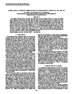
planned), or on large-scale test problems. The full multi-year scheduling concept will be exercised operationally once the scientific program of the telescope is redefmed in mid-1991. The performance of the neural network based on tests with real HST observing. programs has been extremely promising. The scheduling of 2,600 scheduling units consisting of about 12,000 exposures takes less than one hour on an Texas Instruments Explorer IT workstation (Fig. 7-2). A problem of this size represents about six months of HST observing scheduled at one-week time resolution. Scaling with problem size is empirically approximately lin­ ear in the .number of subintervals considered, and quadratic in the number of activities to schedule. This is fast enough to permit the exploration of many potential schedules bef0 (see Eqn. 5-1).

Appendix C:

Stochastic algorithms

The fact that most interesting combinatorial optimization problems are NP-hard - a propeny related to an algorithm executing on a serial, deterministic Turing machine - has motivated recent research in parallel and stochastic algo. rithms. While the use of random numbers is very natural in computer simulations of random processes, the idea of embedding elements of stoehasticity into an algorithm for solving deterministic combinatorial problems is less ob­ vious, but is slowly penetrating the computer science community and has recently become even quite popular (see e.g. Andreatta et al. 1986). Sometimes a simple randomization of the input is sufficient to achieve a considerable speed-up compared to the truly deterministic algorithm (Maffioli 1987a). The perhaps most famous examples of stochastic algorithms are two related methods for testing the primality of in­ tegers proposed independently by Rabin (1976, 1980) and by Solovay &. Strassen (1977): they output uprime" when­ ever the input number is prime, but outputeither uprime" or ucomposite" with some stateable (bounded) probability, when the input is composite. In other words: the output "composite" is always correct, the output uprime" is mostly. The statistical behavior of the primality testers is characterized by the four ttansition probabilities or likelihoods (only two of which are independent) . Pr(primeoutlprimem) = 1

Pr(compositeoutlprimem) = 0

Pr(primeoutlcompositem) = £

Pr(compositeoutlcompositem) = 1 - £

By repeating the algorithm a number of times one can efficiently test even large numbers for primality to any desired certai{1ty, even when £ is not small. The primality testers are typical examples of stochastic algorithms of the Monte Carlo-type which always tenninate in polynomial time, but sometimes lie, as opposed to Las Vegas-type algorithms which always tell the truth, but sometimes fail to stop (see Johnson 1984). Thus Las Vegas algorithms appeaI to those who prefer failure to tenni­ nate to an unreliable answer. A general Monte Carlo algorithm for a decision poblem can be viewed as a probabilistic classifier (Fig. C-l) sorting problem instances from two classes Am and Bin into one of two classes Aout and Bout with likelihoods

=0

Pr(AoutIAm) = 1

Pr(BoutlAm)

Pr(AoutIBm) = £

Pr(BoutlBm) = 1 - £

which depend on the problem's and algorithm's characteristics.

-21­

In practic:aI applications, o~e is no~ so much interested in the likelihoods, but in the posterior probabilities, which allow to mfer the probable mpu~ gIven the somewhat uncenain output The posterior probabilities can be computed from the likelihoods and the probability distribution of the input instances via Bayes theorem of statistics Pr{AinrAouu

= Pr(AoutIAm) Pr(Am) / Pr(Aouu =' Pr(Am) / [Pr(Am) + £ Pr(BirJ]

Pr{BinJAouu

= Pr(AoutIBm) Pr(Bm) / Pr(Aouu = £ Pr(Bm) / [Pr(Am) + £ Pr(Bm)]

Pr(AinIBout}

=Pr(BoutIAm) Pr(Am) / Prd

Vr.r~lIon Of

YllOP 1 11 (TrUl3 'enlon Of VI LOP 6 11

fJ. ur.1 Nrhtort

71 F r.b 90

OI~.IIIlY

mmm~mi! ~ ...•............

..•............

.....•......... .......... .•... ..

..............•

mmmHim;

• •C·5H20710 I

aD. 0 II,.: 3.0010)

• wC·5H207l02

ab. 0.11'•. 300(01

................................

...................

....~--~-+

......................................................................................

.wC·su-0225703

aD•. D.Ii,.: 1.00101

IItlwC·SU-D225704 aD, o.u,. 100(01

.........................._

~_

.

• •C·SUo0207l03

SI,.

all,: 0 3 00(01 SEGtotENTATIOH-II Type FULL

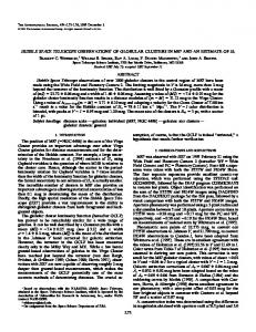
Fig. 7-1: A sample screen showing SPIKE scheduling windows for a small number of activities. The two larger windows display suitability functions for several activities (the one at the bottom is simply a view at higher time resolution). The smaller superimposed window shows a graphical display of the neural network for the same activities: darker squares represent neurons in their "on" state. The displaced row on the right displays "guard" neurons which attempt to ensure that each activity is scheduled at some time.

- 36·

Neural Network Search Timings 1000

100

17

I

I

I

I

I

..J

V

I

'7

/1

I I

10

I

I

I 26HO~X

.1/

/l.&

I'

Elapsed time (minutes)

)~ ~

I

I

52MQJlX

o

26 aeg XII

I

- Appro. tit

JI

~/

/ ' r1V7

I

~//~

0.1

.... ~~

. /V /

0.01

L.--'"

I

:"v

I

I

I

!

!

I

)

.

"

I

I

!

i

IV

0.001

10

I

I

I

[

I

I

I

+

I

!

1000

100

!

I

I ;

;i:

I

; I

10000

• scheduling units

Fig. '-2: Performance of the neural network as a function of problem size. The open squares show the wall­ clock time in minutes as a function of problem size (number of scheduling units) when run on a TI Explorer II workstation (XII): 3000 scheduling units represent about six months of HST scheduling, which can be accomplished in about an hour. The dark line shows the approximately quadratic scaling behavior with problem size. The diamonds represent runs made on TI MicroExplorer (JJ.X) showing scheduling over six months (26 segments) and one year (52 segments) at one-week resolution.

a

-37­

(a)

(b)

Sj(t)

0 (c)

~

\J

Sja(t)

0 t

~

~

Fig. A-I: Illustration of suitability functions for the case of a binary interval preference constraint: (a) Bja(t;ti) represents the suitability of scheduling Aj at t given that Ai is scheduled at ti. The duration of Ai is di and Aj is constrained to stan no sooner than x and no later than x+y after the end of Ai; (b) hypothetical suitability of Ai at some point in the scheduling process; (c) the resulting suitability of Aj- The intervals where each displayed function is non-zero are indicated by bars under the time axis in (b) and (c).

.38 ­

o o

AZ

o

o

=

Fig. B-la: A fragment of the constraint graph G (V, A) of the lOy scheduling problem for N=4. Suppose that activity A} is already scheduled at time tl. The inhibitory edges shown implement the constraints that 1. activity A] should not be scheduled twice by complete lateral row inhibition, that 2. no other activity should be scheduled at time t] by complete lateral column inhibition and that 3. no other activity should occur on one of the two timetable diagonals coincident with place 0,1) by complete lateral diagonal inhibition.

-39·

o AZ

o

Fig. B-lb: Another fragment of the constraint graph G = (V, A) of the toy scheduling problem for N=4, imple­ menting the outbound constraints for activity A2 assumed It> be scheduled at time t2.

.40­

o

AZ

• • •

o • • • t,

• •

o

• • • o •

Fig. 8-2a: A globally optimal (K = N) solution for the N=4 toy scheduling problem.

- 41­

o

• • • o

• • • • • • • o

• • •

Fig. B·2b: A feasible configuration of our toy scheduling problem for N=4, corresponding to an attractive stable fixed-point of the network dynamics, which cannot be extended to a globally optimal (K = N) solution by placing activity A3 somewhere.

-42·

AZ

Fig. B-3: An additional network of fast "hidden" guard neurons asymmetrically coupled to the main network al­ lows the implementation of the global constraint that only globally optimum (K N) configurations of the original problem are feasible.

=

.43·

Proba bilistic classifier

.-

,

......

• " "- " " " "

""

­

)(

Bout

-

......

¥ "

•

""

"

4

Fig. e-l: Solving instances of a binary decision problem with the help of an unreliable probabilistic classifier: being fed with a problem instance the classifier decides upon either of two output categories, where sometimes this decision is erroneous. Nevertheless, by repeating the classification process sufficiently often the uncertainty about the true category of the problem instance can (in a probabilistic sense) be made arbitrarily small. In a sense the ODS-network when acting on a CSP can be likened to a probabilistic classifier.

-44-

Biographies Dr. Mark D. Johnston is an Associate Scientist at the Space Telescope Science Institute (STScI) where he is Deputy Head of the Science and Engineering Systems Division. He was responsible for the design and development of both the Proposal Entry Processor and SPIKE scheduling system. He received his Ph.D. from M.I.T. in 1978 with a thesis on High-Energy Astronomy Observatory (HEAD-I) X-ray observations of the Large Magellanic Cloud. He has extensive experience with satellite data and has authored or co-authored 30 papers based on the analysis of HEAo-l X-ray data. His other research interests include numerical hydrodynamics, nucleosynthesis in supernovae. statistics and classification techniques. and the application of advanced software and computing techniques to astronomical research. In recent years he has authored or co-authored about 20 papers in these areas. He was an Assistant Professor of Astronomy at the University of Virginia before moving to STScI in 1982. . Hans-Martin Adorl, a theoretical physicist by education. has been working in astronomy since 1980. In 1985 he joined the Science Data and Software Group of the Space Telescope - European Coordinating Facility. where he is employed as data analysis scientist within the Hubble Space Telescope project. He is one of the founders of the uST-ECF Artificial Intelligence Pilot Project" and has· sporadically participated in the SPIKE project. While the center of gravity of his professional work has recently shifted to HST image restoration, he maintains an active interest in the application of AI techniques to astronomical problems. He has authored or co-authored more than 35 papers in the area of expert systems. neural networks. databases, observatory operations, data analysis, statistical pattern recognition and classification of astronomical objects.