ScienceDirect Optimization of PID Control for High

Available online at www.sciencedirect.com

ScienceDirect Procedia Computer Science00 (2015) 000–000 www.elsevier.com/locate/procedia

2015 IEEE International Symposium on Robotics and Intelligent Sensors (IRIS 2015)

Optimization of PID Control for High Speed Line Tracking Robots. Vikram Balajia*, M.Balajib, M.Chandrasekaranc, M.K.A.Ahamed khand, Irraivan Elamvazuthie a

b

Final Year,Department of ECE,Government College of Engineering Salem,India.

Technical Director,Frontline Electronics Pvt.Ltd,Salem,India. ECE, c Professor and Head,Department of ECE,Government College of Engineering Bargur,India. dFaculty of Engineering,UNISEL 45600,Kuala selangor,Malayisa. eUniversity Technologi PETRONAS31750,Malaysia.

Abstract The paper focuses on the optimization of the classical PID control technique for implementation in a high speed line tracking robot. The control technique is tested on a prototype line tracking robot, which uses an array of ten Infra-Red reflective sensors to track a non-reflective line on a reflective surface. The paper describes in detail the various challenges that are specific to the mobile robot line tracking system and the adaptation of PID control to successfully control the highly non-linear and unstable system. Various forms of PID control are implemented and the merits and demerits of the same are discussed. A customized PID control implementation scheme is proposed which combines the aspects of closed loop PID control and open loop control. © 2015 Vikram Balaji. Published by Elsevier B.V. Peer-review under responsibility of organizing committee of the 2015 IEEE International Symposium on Robotics and Intelligent Sensors (IRIS 2015). Keywords: Mobile Robots; Line Tracking; PID Control; Differential Drive.

1. Introduction Line Tracking is one of the most useful and popular behaviour of mobile robots that has been acquiring increasing importance in the recent times. Line tracking has become the most convenient and reliable navigation technique by which autonomous mobile robots navigate in a controlled, usually indoor environment. The path of the robot is demarcated with a distinguishable line or track, which the robot uses to navigate. Commonly used examples of these lines include magnetic tape on a non-magnetic surface, a void or a cut on a flat surface, a reflective tape on a non-reflecting surface and vice-versa. In most of the situations, the robots are mounted with Hall-Effect sensors or Photo-interrupters, which are based on Infra-Red or visible light.

1877-0509© 2015 Vikram Balaji. Published by Elsevier B.V. Peer-review under responsibility of organizing committee of the 2015 IEEE International Symposium on Robotics and Intelligent Sensors (IRIS 2015).

Vikram Balaji / Procedia Computer Science00 (2015) 000–000

2

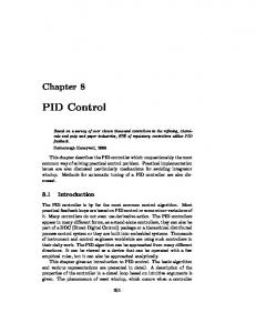
Traditionally, the approach to line tracking is usually considered in the digital domain where the outputs from the digital line sensors are given to a microcontroller which is programmed to run the motors of the robot in various speeds depending on where the robot is positioned with respect to the centre of the line [1] - [6]. The motor speed settings are selected by trial and error for various sensor readings. While this approach has the advantage of being very simple, it is usually not very convenient due to the following limitations. 1) Programming becomes increasing difficult when the speed has to be increased beyond 25 to 30 centimeters per second for a small sized indoor robot. 2) The addition of more sensors further increases programming complexity. 3) Re-tuning is needed when the line thickness has to be varied. 4) Program development time is very large and requires considerable experience in robotic programming to create reliable performance. 5) When digital sensors are used, the sensor state changes occur only when the deviation in robot position is greater than the gap between the sensors. The natural response is to change the motor speed drastically, which results in the robot making the jerky movements. This is undesirable in many applications. All the above mentioned issues can be solved by using analog line sensors for detecting the line [7], [8] and by using automatic control techniques for manipulating the motor speeds [8-10]. 2. The Test Platform 2.1 The Basic Hardware The test robot is a two-wheeled mobile robot with differential drive. A ball castor provides third point contact to ensure stability. The robot is driven by two high speed miniature permanent magnet gearmotors coupled to wheels. The robot is battery powered, with the motors supplied with regulated power supply to ensure consistent motor power at all operating scenarios. The robot can reach a maximum speed of about 130 cm per second. Photos of the test platform are shown in Fig. 1 and Fig. 2. To move the robot forward, both motors are rotated in the forward direction. To make the robot turn to the left or to the right, the speed of one motor is reduced. The amount of turn increases as the speed difference increases. Maximum amount of turn is achieved when one motor is turned in a backward direction at maximum speed. This results in maximum speed difference and the robot just spins in place. The brain of the robot is an R8C25 16-bit microcontroller from Renesas. Bidirectional motor speed control is achieved by using an H-Bridge motor driver circuit. The power applied to the motor is varied by using PWM generated by the microcontroller. 2.2 The Line Sensors The robot has an array of ten analog IR (Infra-Red) reflective photointerrupters to detect a non-reflective (Black) line on a reflective (White) surface. The sensors are placed at gaps of 10 mm and the total sensor coverage is 90 mm. The sensor array is placed in front of the robot and can be seen in Fig.3.

Fig. 1. Front View of the Robot

Fig. 2. Side View of the Robot

Fig. 3. Sensor Array of the Robot

Each reflective photointerrupter consists of an IRED (IR LED) and an IR Phototransistor. The IR rays emitted by the IRED fall on the surface. If the surface is reflective (White), the IR rays are reflected back to the IR Phototransistor which conducts current. So, the potential difference across the device is reduced. Otherwise, if the


3

surface is non-reflective (Black), the IR rays are absorbed and the IR Phototransistor remains non-conductive which results in a high potential difference across the device. All the sensors are connected to the ADC ports of the microcontroller. Since IR sensors are extremely sensitive to interference from external light sources, notably incandescent lamps and sunlight, the sensor array is covered on the top and the sides with black colored sheets to block out external light interference. This can be clearly seen in Figure 3. 2.3 Calculation of Positional Error from Sensor Data The output of the IR line sensor array is fed to the microcontroller which calculates the error term from sensor values. The most convenient and reliable way to compute the error term is by dividing the weighted average of the sensor readings by the average value and normalizing the values. The formula used is given as follows: Error e(n) = 1000 ×

∑ ∑

∗

– 4500

th

In the equation, Lx refers to the output of the x line sensor in the array. Here, 1000 is the normalizing factor which is used to ensure that the contribution of the error term from each sensor is normalized to a value of 1000. The subtraction by 4500 is to ensure that zero error occurs when the robot is centered on the line. The sensors are numbered from the left to the right. An error value of zero refers to the robot being exactly on the center of the line. A positive error means that the robot has deviated to the left and a negative error value means that the robot has deviated to the right. The error can have a maximum value of ±4500 which corresponds to maximum deviation. The main advantage of this approach is that the ten sensor readings are replaced with a single error term which can be fed to the control algorithm to compute the motor speeds such that the error term becomes zero. Further, the error value becomes independent of the line width and so the robot can tackle lines of different thicknesses without needing any change in code. 3. Characteristics of the Line Tracking Control System 3.1 Mechanical Characteristics The robot is driven by DC gearmotors which are coupled to wheels. The motor speeds are controlled by adjusting the mean voltage supplied to the armature by using PWM. Although, the motor speed increases with increase in applied voltage, the relationship is non-linear. The dynamic load on the motors, the robot weight and inertia, further increases the non-linearity. Although both motors are similar, slight mechanical differences in the motors usually results in the motors rotating at different speeds even when equal power is applied. This causes the robot to drift towards the right or left instead of moving forward. Due to the non-linearity in the speed of the motors, the robot path deviation is different at different motor speeds. The constraints due to the motors remain as one of the most significant and defining characteristic which affects the performance of the entire system. 3.2 Sensor Characteristics IR photointerrupters, which are used as the line sensors are themselves non-linear, i.e. the sensor values are just an indication of surface reflectivity. The sensor value is lower when over a white surface and higher when over a dark surface. The actual values are heavily dependent on the external lighting conditions even though sensor array is shielded. Further, there is appreciable difference between the readings of various sensors due to various factors like placement, manufacturing differences, etc. To get usable values from all the sensors, the sensor values are normalized for environmental conditions and sensor differences and the normalization values are stored in Data Flash of the microcontroller. This enables the normalization data to be used multiple times. To normalize the sensor values, the robot is placed on the track and rotated such that all the sensors pass over the black and white surfaces. The maximum and minimum readings for all the sensors are noted down and stored in non-volatile memory (Data Flash) of the microcontroller. When the positional error value is to be calculated, the sensor readings are scaled to a normalized value between 0 and 1000 such that 0 corresponds to the minimum value (White) and 1000 corresponds to the maximum value (Black). Thus, the sensor readings are normalized such that when all the sensors are placed over any surface with uniform reflectivity, a uniform value is obtained from all of them.

4


The usage of normalized sensor values to calculate the sensor error value results in a fairly accurate error parameter, notably when all the sensors are exactly over the black or white surfaces and none of them are in the transition region between the two surfaces. However, when one or more sensors are at the edge of the transition region between the two surfaces, the error parameter becomes non-linear because of the inherent non-linearity of the sensor values with respect to surface reflectivity. This is a very important aspect of the system because random errors are expected in the sensor error parameter. Since the errors are due to non-linearity, there is nothing else that could be done to remove them. This is also different from traditional control systems where feedback is taken from a sensor which directly measures the output of the plant. Any error that occurs is usually due to noise which can be removed by using specific filters. Unfortunately, this technique is not applicable for the line tracking system. These unavoidable random errors cause a lot of issues in control system implementation. 3.3 Input and Output Considerations The objective is to make the robot move forward at high speed and maintain its course such that the sensor error parameter is zero, (i.e.) the center of the robot coincides with the center of the line at all times. The following can be stated as the considerations for the input and output of the system. 1. The width of the black line shall be at least 2 cm so that least two line sensors will see the line at any instant [6]. 2. The set point of the system is always zero (i.e.) being in the centre of the line is always the objective. 3. The path of the robot, which is marked by the black line, can have straight lines, smooth curves and abrupt turns including right angled and acute angled turns. 4. The robot is expected to track the line faithfully without any problems. The robot should not leave the line at any instant. 5. The movement of the robot should have minimum overshoot and all the movements should be smooth. 6. Exact maintenance of the sensor error parameter at zero value is not feasible even in a straight path because of the random errors due to sensor non-linearity and changes in ambient light conditions. An error of 5 to 10 percent is considered acceptable. 7. Traditional performance specifications like MSE(Mean Square Error), ISE(Integral Square Error), ITAE(Integral Time Absolute Error) are not applicable for this system because of the random errors in sensor values. The only meaningful performance specification is the time taken to traverse a standard test track. It is assumed that, for a constant motor speed setting, the controller setting which achieves the minimum MSE, traverses the path in the shortest time. This is justified because when the error is more, the correction will naturally be more, which causes the speed of the robot to be reduced. 4. Characteristics of the System From a Control System Perspective 4.1 Steady State Error and System Type The steady state error of the system is usually used for characterization of the system based on its type (i.e.) Number of integrators in the feed-forward path. A closed loop unity feedback system is considered, in which the control effort is the error multiplied by a gain. This is similar to proportional control. A test of steady state error is made by counting the number of overshoots to the left and to the right. Initially, the robot is started with the maximum amount of deviation such that the sensor error parameter is 4500 or -4500. When the robot is placed on a straight track, it is seen that the robot oscillates on both sides by an equal amount. This proves that the steady state error is zero for a straight line. When the robot is placed on a curved track, it is seen that the robot overshoots the line centre by a greater amount in the direction opposite to the direction of curvature of the track. Further, it was observed that, as the curvature increases, the difference in overshoots increases. This proves that a steady state error exists when the track is curved. For the system, it was stated that the setpoint is always zero (centre of the line) but the line may not be a straight line. So the line curvature may be considered as an external disturbance to the system. Now, it can be concluded that, when the system has zero or negligible disturbance (analogous to a step input for a simple unity feedback system), the steady state error (position error) is zero. When a significant disturbance exists (analogous to a ramp or parabolic input for a simple unity feedback system), the steady state error (velocity and acceleration errors) are


5

significant values. From the above discussion, it can be concluded that the system under consideration is of Type 1 or greater type. This means that there are multiple integrators in the feedforward path of the system and that the controller design is therefore non-trivial [11]. 4.2 Open Loop Characteristics and Loop Type Consider an open-loop test on the line tracking system. The system characteristics can be better understood by considering the following conditions. 1) Assume that the robot is placed exactly on the centre of a straight line and exactly in the direction of the line. If no control effort is exerted (both motors run at equal speed), the robot moves forward with zero error. This is the only special condition where zero control effort is needed. 2) If there is any discrepancy, line not being exactly straight, robot not being perfectly aligned or the existence of speed difference between the motors, control effort is needed (speed of one of the motors must be reduced). 3) Now, assume that the robot is away from the centre of the line by some distance. In order to reduce the error, a control effort must be given. However, the exertion of a constant control effort will cause the robot to overshoot the line. From the above considerations, it can be understood that the loop is integrating (i.e.) control effort is being integrated by the system [12]. The open loop response of the system thus resembles that of a servo position control system. Thus, the control techniques used for servo control may be applicable for the line tracking robot. The most popular control technique for servo position control, the PD controller will be a good starting point for the design of the controller for the system. 5. The Classical PID Controller The system has been tested initially with the classical PID controller implemented in parallel form. The well known PID controller equation is shown here in continuous form. ( )=

× ( ) +

×

( )×

+

×

( )

Where kP, kI and kD refer to proportional, integral and derivative gain constants respectively. For implementation in discrete form, the controller equation is modified by using the backward Euler method for numerical integration. The term which represents the sampling time, tS is simply eliminated because of multiplication with constant values (i.e.) the PID gains kI and kD. ( )= where

=

×

and

× ( ) +

×

( ) +

×

( ) − ( − 1)

=

The motor speeds are set depending on two parameters; the PID controller output and the maximum motor power, which determines the speed at which the robot is running. The motor speed equations are given as If the sensor error parameter is negative, ( )= ( )= + ( ); _ If the sensor error parameter is positive, ( )= ( )= _ ; _ − ( ) From the above equations, it can be clearly seen that when the robot deviates to the right (negative error parameter), the left motor speed is reduced to make the robot move to the left. Similarly, when the robot deviates to the left (positive error parameter), the right motor speed is reduced to make the robot move to the right. Another notable point is that, when the sensor error parameter is negative, the controller output usually will also have the same polarity. So, for negative error parameter, the controller output c(t) is added to the left motor speed setting. The step-by-step implementation of classical PID controller is explained along with the issues that made it unsuitable for the line tracking system.


6

5.1 The Proportional Only Controller Initially, a simple proportional controller was tested with a straight line. It was seen that the robot oscillates greatly to the left and to the right while tracking the line and the transient response was considerably slow. Increase of the Proportional Gain KP improved the speed of the transient response but the oscillations became worse. Decreasing the gain reduced the oscillations but at the cost of more sluggish transient response. The performance became even worse when the straight line was replaced by a curved path because of the addition of steady state error. The simple P-controller was not suitable for the system. So, the derivative and integral terms were added to improve the performance. 5.2 The Addition of Derivative Control In PID control, the derivative term is used to reduce the overshoot and to improve the transient response. But, the derivative term is extremely sensitive to noise in the sensor readings. Since the sensor error term is affected by random errors due to non-linearity, the derivative gain had to be kept low in order to prevent rapid motor speed changes. With this PD controller, the line tracking system performance is fairly satisfactory for straight lines. But for curved paths, the performance was not very satisfactory due to steady state error. As a result, the overall motor speed had to be reduced for the robot to be stable when negotiating turns and curves. This reduced overall robot speed. 5.3 The Addition of Integral Control Integral term is usually used to reduce steady state error in a control system. Addition of the integral term reduces steady state error when the path is a simple curve. But, when the path is made up of various curves, straight lines and turns, integral control action becomes problematic. Normally, integral control action is used to reduce steady state error due to a constant disturbance (like friction in a motor speed control system). But in this system, the disturbance due to line curvature is not constant because the line characteristics changes continuously. So, direct implementation of integral control is not effective. It can hence be concluded that Classical PID control is not suitable for implementation for the line tracking system. Certain modifications are needed to adapt the PID control scheme to make it suitable for the system. 6. The Optimized PID Controller Implementation In order to suitably implement the PID controller, the following modifications were made to implementations of integral term along with a few other modifications to improve performance. 6.1 Modified Integral Control Implementation The implementation of the Integral Term in Classical PID controller was unsuitable for line tracking robot because of the problems when the curvature of the line changes. In order to solve this problem, only the last ten error values are summed up instead of adding all the previous values. The modified controller equation is given as ( )=

× ( ) +

×

( ) +

× ( ( ) − ( − 1))

This creates an integral control effort that strives to counteract steady state errors in curved paths, but is also adaptive to changes in curvature of the track. This technique provides satisfactory performance for line tracking. 6.2 Addition of Speed Variation Parameter For stability considerations, the maximum speed of the robot had to be set depending on the characteristics of the track on which the robot runs. This reduces the average speed of the robot because the speed needs to be reduced so that the robot is stable when negotiating sharp curves. In order to avoid this problem and to improve performance, the speed of the robot needs to be dynamically changed depending on curvature of the track. To achieve this, an additional parameter has been introduced which is henceforth called the speed reduction parameter. The speed reduction parameter is similar to the modified integral control parameter but it reduces the speed of both motors. The equation for the speed reduction parameter is given as


( ) =

×

7

| ( )|

So, the modified motor speed equations are given as If the sensor error parameter is negative, ( )= ( )= + ( ) − ( ); _ − ( ) If the sensor error parameter is positive, ( )= ( )= − ( ); _ − ( ) − ( ) Now, the maximum speed of the robot is set so that the robot tracks a straight line with acceptable stability. The speed reduction constant KSR gradually increased until stability is acceptable for curved paths and turns. So, the robot navigates at a higher speed in the straight paths and slows down slightly at turns so that stability is maintained. 6.3 Addition of Open Loop Control for Saturated Condition The above mentioned technique works suitably well for straight lines, curves and moderate turns. However, for sharp acute angled turns, the performance is not acceptable and the robot misses the turn or has excessive overshoot issues. This is due to the fact that, when the path has an abrupt turn, the robot goes entirely off the line causing the sensor error parameter to saturate to values of either 4500 or -4500 depending on the direction of the turn. In this condition, the control effort produced by the modified PID controller will be unable to turn the robot fast enough. To solve this problem, an open-loop control scheme is implemented when the sensor error parameter gets saturated. The robot is rotated in the clockwise/anticlockwise direction by turning one of the motors in the backward direction. This is done until the robot detects the line. Then, normal closed loop control is used. 7. Results In order to test the various algorithms and to validate their performance, a test track was constructed which has all types of turns and curves expected in a robotic competition. The track which can be seen is Fig. 4 consists of the following; a straight path of about 120 cm, a half circle with radius 40 cm, an ‘S’ shaped path consisting of two small half circles in opposite directions of radius 12 cm, One right angled turn and two acute angled turns(400). The robot is assigned a maximum speed setting that will allow reliable line tracking. For each setting, the best possible values for all the parameters are chosen by iterative closed loop tuning techniques as described in [13]. The results are described in Table 1. The experimental results vindicate the theoretical assumptions made in the previous sections. PD control is the first control strategy that provides line tracking without excessive overshoot, but maximum speed is limited to only 90% motor power. Modified PID control reduces overshoot at curves enabling the set speed to be increased to 95%. The addition of speed reduction enables maximum speed setting to be increased to 100% motor power. Speed reduction enables the robot to slow down in turns for better stability. In all the above control strategies, the robot failed to navigate the acute angled turns at the end of the track. The addition of open loop control for saturated condition gives the best performance enabling successful traversal of all track configurations.

Fig. 4. Test track layout


8

TABLE I. Performance of various algorithms

Algorithm

Time Taken (sec)

Set Speed

1

2

3

4

5

P control

2.43

4.96

7.34

9.8

-

80%

PD control

1.56

3.26

5.05

6.74

-

90%

Modified PID control

1.37

2.94

4.57

6.17

-

95%

Modified PID control with speed reduction

1.15

2.68

4.27

5.98

-

100%

Modified PID control with speed reduction and open loop control

0.95

2.51

4.04

5.79

8.3

100%

8. Further Work The following improvements can be made to the test platform to facilitate the implementation of more advanced control strategies. 1) Inclusion of high resolution quadrature encoders for measurement of motor speed and position. 2) Implementation of cascaded motor speed control loop within the main line tracking loop. 3) Implementation of inverse kinematic robot movement control for better performance in line tracking. 4) Usage of machine learning techniques to linearize the sensor error parameter. 5) Implementation of wireless telemetry systems for wireless, real-time data acquisition. 9. Conclusion The optimized PID control scheme implemented in the robot proved successful and allowed the robot to negotiate a non-trivial track with the highest speed possible. The robot moves with a maximum speed of about 120 cm per second. The control algorithm gives acceptable performance and is suitable for implementation in a scaledup robotic system for various real-world applications. References [1] [2] [3] [4] [5] [6] [7] [8] [9] [10] [11] [12] [13]

Borcoşi, Ilie, Luminiţa Popescu, and Daniela Nebunu. "Line tracking robot." In International Conference on Manufacturing Systems ICMaS, Bucuresti, pp. 26-27. 2006. Colak, Ilknur, and D. Yildirim. "Evolving a Line Following Robot to use in shopping centers for entertainment." In Industrial Electronics, 2009. IECON'09. 35th Annual Conference of IEEE, pp. 3803-3807. IEEE, 2009. Bajestani, Seyed Ehsan Marjani, and Arsham Vosoughinia. "Technical report of building a line follower robot." In Electronics and Information Engineering (ICEIE), 2010 International Conference On, vol. 1, pp. V1-1. IEEE, 2010. Pakdaman, Mehran, M. Mehdi Sanaatiyan, and Mehdi Rezaei Ghahroudi. "A line follower robot from design to implementation: Technical issues and problems." In Computer and Automation Engineering (ICCAE), 2010 The 2nd International Conference on, vol. 1, pp. 5-9. IEEE, 2010. Punetha, Deepak, Neeraj Kumar, and Vartika Mehta. "Development and Applications of Line Following Robot Based Health Care Management System." In Advanced Research in Computer Engineering & Technology (IJARCET), 2013, International Journal of, vol 2, issue 8, August 2013 Baharuddin, M. Zafri, Izham Z. Abidin, S. Sulaiman Kaja Mohideen, Yap Keem Siah, and Jeffrey Tan Too Chuan. "Analysis of Line Sensor Configuration for the Advanced Line Follower Robot." Huang, Hsin-Hsiung, Chyi-Shyong Lee, Juing-Huei Su, Chia-Lung Yang, and Tsai-Ming Hsieh. "Industry-‘Orientation Training Course by Line Following Maze Robot." International Journal of Education and Information Technologies (2011): 105-112. Lee, Chyi-Shyong, Juing-Huei Su, Kuo-En Lin, Jia-Hao Chang, and Gu-Hong Lin. "A project-based laboratory for learning embedded system design with industry support." Education, IEEE Transactions on 53, no. 2 (2010): 173-181. Chan, “Desktop line-following robot,” Accessed May. 26, 2015 [Online]. Available: http://elm-chan.org/works/ltc/report.html Pratheek.N, “An advanced line following robot with PID control,” Society of Robots, Accessed May 26, 2015 [Online].Available: http://www.societyofrobots.com/member_tutorials/book/export/html/350. Ogata, Katsuhiko, “Modern Control Engineering” 5th ed. Pearson Education Inc. Peacock, Finn, “PID Control Blueprint V2.0” 2008, eBook, [Online] .Available: http://www.pidtuning.net Ledin, Jim, “Embedded Control Systems in C/C++”, CMP Books.