ScienceDirect - syscop

A Schur Complement Method for Optimum Experimental Design in the Presence of Process Noise ? Adrian B¨ urger ∗,∗∗ Dimitris Kouzoupis ∗∗ Angelika Altmann-Dieses ∗ Moritz Diehl ∗∗,∗∗∗ ∗ Faculty of Management Science and Engineering, Karlsruhe University of Applied Sciences, Germany ∗∗ Department of Microsystems Engineering, University of Freiburg, Germany ∗∗∗ Department of Mathematics, University of Freiburg, Germany

Abstract: Optimization problems arising in Optimum Experimental Design (OED) applications require repeated covariance matrix evaluations of the underlying Parameter Estimation (PE) problems. The complexity of this task grows quickly with the problem dimensions, especially when process noise is considered. In this paper, a Schur complement method is proposed to alleviate this problem by translating the covariance matrix evaluation into the solution of a sparse linear system and the inversion of a small-scale matrix. The method is used as a building block for the open-source software package casiopeia, a powerful and easy-touse environment for OED and PE. The performance of the software and the proposed Schur complement method is assessed on a numerical example. Keywords: Input and excitation design, Software for system identification 1. INTRODUCTION In Parameter Estimation (PE) problems, the amount of information that can be extracted on the unknown parameters strongly depends on whether the conducted experiment was able to sufficiently excite the relevant system dynamics. A useful indicator for assessing the quality of the estimation results is the covariance matrix of the estimated parameters, see e. g. Walter and Pronzato (1997), Pronzato (2008). High values for a parameter’s variance indicate that the setup was not optimal for determining its true value – even if the fitting to the given measurements is satisfactory – since either the inputs of the system were not well designed or the adopted model was inadequate. High covariance values may for instance occur when the values of some model parameters strongly depend on the values of others. Since it is favorable not only to evaluate the information content of one experiment, but to ex ante determine meaningful experimental setups to reduce effort and cost, the covariance matrix is further used within Optimum Experimental Design (OED) to design experiments that result in a higher confidence on the estimated parameter values 1 (Pronzato, 2008), (Bock et al., 2013). In OED, the ? Support by the EU via ERC-HIGHWIND (259 166), ITN-TEMPO (607 957), and ITN-AWESCO (642 682), by DFG in context of the Research Unit FOR 2401 and by Ministerium fuer Wissenschaft, Forschung und Kunst Baden-Wuerttemberg (Az: 22-7533.30-20/9/3) is gratefully acknowledged. 1 Other OED approaches aim at minimizing the cost of the identification experiment while guaranteeing an acceptable control performance, see e. g. Annergren (2016).

covariance matrix is part of the objective of an optimization problem, which makes the efficient evaluation of the matrix crucial and every increase in computational effort problematic. Different approaches exist to calculate and use the covariance matrix in this context, see e. g. Bauer et al. (2000), K¨orkel (2002), K¨orkel et al. (2004), Bock et al. (2007), Kostina and Kostyukova (2012). If a system is subject to noise that affects its dynamics and this noise is not explicitly considered within the PE problem, the estimation results may be inaccurate. As a remedy to this, additional degrees of freedom can be introduced in the PE problem formulation that capture such process noise and improve the estimation results. This approach is customary in the field of optimization based state and parameter estimation, see e. g. Rao et al. (2003). However, these additional degrees of freedom increase the effort to evaluate the covariance matrix, which can in turn have a negative impact on the solution times of OED problems. Within this paper, a method to compute the covariance matrix based on the Schur complement is presented, which relies on the solution of a sparse linear system and the inversion of a small-scale matrix (with dimension equal to the number of estimated parameters). Although the method is presented for the case of process noise, it is deliberately kept generic and thus applicable to other types of noise as well. To facilitate direct use within PE and OED applications, the open-source software package casiopeia that contains an implementation of the proposed method is introduced and its performance is assessed on a numerical example.

The paper is organized as follows. Section 2 shows how the consideration of process noise increases the effort to compute the covariance matrix for both unconstrained and equality constrained parameter estimation problems. In Section 3 the Schur complement method for the covariance matrix evaluation is presented. The requirements for using this approach within OED are discussed in Section 4. Finally, casiopeia is introduced in Section 5 and its performance is assessed in the numerical case study of Section 6. 1.1 Notation In the following, the accent a ¯ is used to denote a variable that is fixed within an optimization problem. The accent e a means that the variable is polluted by noise and a ˆ that it is the solution of an optimization problem. 2. COVARIANCE MATRICES IN PARAMETER ESTIMATION In the following, we introduce the notion of covariance matrices in the context of both unconstrained and constrained least-squares PE. Least squares PE is a common method for formulation of linear and nonlinear PE problems, see e. g. Nocedal and Wright (2006). Further, we show how the consideration of process noise increases the computational effort to evaluate the covariance matrices.

as in Bauer et al. (2000). In order to obtain an unbiased estimate for the covariance matrix, Σpˆ has to be scaled by a factor

βpˆ =

pˆ = arg min ke y − h(p; u ¯)k2Σ−1 , y

(ˆ p, w) ˆ = arg min ke y − h(p, w; u ¯)k2Σ−1 + kwk2Σ−1 . y

 Σpˆ = 2

∂h (ˆ p; u ¯) ∂p

>

Σ−1 y



!−1 ∂h (ˆ p; u ¯) , ∂p

(4)

 ∗ >  −1 !−1 ∂h∗ ∂h 0 Σy (ˆ v; u ¯) (ˆ v; u ¯) (5) 0 Σ−1 ∂v ∂v w

    with v > = p> w> ∈ Rnv and h∗ (·)> = h(·)> w> . The scaling factor becomes

βvˆ =

ˆ 2Σ−1 ke y − h(ˆ p, w; ˆ u ¯)k2Σ−1 + kwk w

y

(N − np )

.

(6)

The matrix Σpˆ is now a submatrix of Σvˆ , located at the upper left corner due to the ordering of the optimization variables. The dimensions of Σvˆ are indicated in (7). np

nw

Σpˆ

Σ> p, ˆw ˆ

Σp, ˆw ˆ

Σwˆ

  Σvˆ =  

  np   nw

(7)

This implies that the computational effort for obtaining Σpˆ has increased, despite the fact that the content of the other submatrices of Σvˆ is typically not of interest. 2.3 Covariance matrices for equality constrained problems

(2)

The vector u ¯ contains the vectorized inputs of all time steps. The vector e y contains the vectorized measurements of all time points. The noise of the measurements is assumed to be uncorrelated between time points, but can be correlated for measurements at one time point, i. e., the matrix Σy can be diagonal or block-diagonal.

3

w

The covariance matrix of (4) is now obtained from

np

The covariance matrix can now be used for assessing the quality of the estimation results pˆ of (1) for the experimental setup determined by u ¯. An estimate for this matrix is

(3)

If the system is subject to process noise, additional degrees of freedom w ∈ Rnw can be introduced in the optimization problem to yield more accurate results. For zero-mean Gaussian process noise N (0, Σw ) with (co-)variances Σw ∈ Rnw ×nw , the PE problem becomes

(1)

with unknown parameters p ∈ R and fixed, noisefree inputs u ¯ ∈ Rnu that are applied to the system during a certain experiment. 2 The measurement values ye ∈ Rny are polluted by additive, zero-mean Gaussian noise N (0, Σy ) with Σy ∈ Rny ×ny the (co-)variances of the measurements. 3 The weighting matrix Σ−1 y is the inverse of Σy . The model response h(·) ∈ Rny may e. g. come from a single shooting discretization of a dynamic system, see e. g. Press (2007). It is assumed that the inputs are piecewise constant within one discretization interval and the measurements are taken at the discretization time points.

,

2.2 Covariance matrix evaluation under process noise

Σvˆ =

Consider a possibly nonlinear, unconstrained least-squares PE problem of the form

y

(N − np )

where N is the number of measurements of the experiment. In case (1) is a linear PE problem, βpˆΣpˆ is an unbiased estimator for the covariance matrix of (1) (Ljung, 1999). In case (1) is nonlinear, βpˆΣpˆ is an approximation for the covariance matrix.

 2.1 Evaluation of covariance matrices

ke y − h(ˆ p; u ¯)k2Σ−1

For PE of dynamic systems, it is usually favorable to use multiple shooting instead of single shooting for discretization of the dynamics (Bock, 1983). This results in equality constrained PE problems. Consider the equality constrained least-squares PE problem of the form

minimize ke y − h(p, x, w; u ¯)k2Σ−1 + kwk2Σ−1 y w p, x, w subject to g(p, x, w; u ¯) = 0,

(8) n×n

with g ∈ Rng coming from a multiple shooting discretization of a dynamic system. Vector x contains the optimization variables introduced for the system’s states.   Let z > = p> x> w> be the concatenation of the optimization variables and B(·) the Hessian approximation of the Generalized Gauss-Newton method (Bock, 1983). We define the Karush-Kuhn-Tucker (KKT) matrix K of (8) as   B(z; u ¯) gz (z; u ¯ )> K(z, u ¯) = , (9) gz (z; u ¯) 0 with gz (·) the Jacobian of g(·) with respect to z. The covariance matrix Σzˆ of the equality constrained leastsquares PE problem in (8) is now equal to the upper left submatrix of K −1 , i. e., nz 

K

−1

 M11 (ˆ z; u ¯) =  M21

ng

with A ∈ R unknown as in

n×m

, C ∈ R

known and X ∈ R

X = solve(A,C).

(14)

Then, solve() can be used to directly compute Σpˆ as Σpˆ = Zp> · solve(K,Zp ).

(15)

without explicitly computing K −1 beforehand which reduces the computational effort significantly, see e. g. Golub and Loan (1996). The multiplication with Zp> is only a selection of elements from solve(K,Zp ) and therefore it introduces no additional computational cost. Further gain in efficiency is obtained if solve() can exploit the sparsity of the involved matrices.

> n M21  z  ng M22

When K is partitioned as (10) np 

 K11 K= K21

In this section, an efficient approach is presented to obtain Σpˆ from K using the Schur complement. 3.1 Efficient matrix inversion using linear solvers In principle, Σpˆ can directly be obtained from K −1 as Σpˆ = Zp> (K −1 Zp ),

(11)

with Zp being a projection matrix from K −1 to Σpˆ, i. e., np

(nz − np + ng )  > np K21   (nz − np + ng ) K22

(16)

the Schur complement can be used to compute the covariance matrix Σpˆ, which corresponds to the upper left block of the inverse of (16), as

3. COVARIANCE MATRIX EVALUATION VIA A SCHUR COMPLEMENT METHOD

−1 > Σpˆ = (K11 − K21 (K22 K21 ))−1 .

(17)

Note that K22 is invertible if the Nonlinear Programming (NLP) problem that corresponds to the problem with all parameters p fixed, satisfies the Second Order Sufficient Condition for local optimality (Nocedal and Wright, 2006). This assumption corresponds to a well-posed parameter estimation problem and it is for example the case when the constraints come from a multiple shooting discretization and the disturbances are penalized with positive definite weighting matrices. 5 −1 Again, it is crucial to compute (K22 K21 ) at once using the previously introduced solve() operator. In this case, Σpˆ is evaluated as



n  I  p  Zp =  nz + ng − np 0

> Σpˆ = (K11 − K21 · solve(K22 ,K21 ))−1 .

(12)

and I ∈ Rnp ×np the identity matrix. For this calculation to be efficient, it is crucial not to explicitly calculate K −1 , but to evaluate (K −1 Zp ) directly. Consider a numerical (or symbolic) linear solver solve() that is able to solve a linear system of the form 4

(13)

n×m

3.2 Inversion of submatrices using the Schur complement 

with Σzˆ = M11 (Kostina and Kostyukova, 2012). Note that Σzˆ contains all (co-)variances for all optimization variables z. Again, due to the ordering of the variables p, x, and w in z, only the upper left submatrix Σpˆ of Σzˆ contains relevant information on the quality of pˆ. For a multiple shooting problem (8) and a corresponding single shooting problem (4), the resulting covariance matrices Σpˆ coincide. 4



AX = C,

In single shooting, w also contains degrees of freedom for estimation of the initial states.

(18)

In order to obtain an unbiased estimator, Σpˆ needs now to be scaled by the factor

βzˆ = 5

ke y − h(ˆ p, x ˆ, w; ˆ u ¯)k2Σ−1 + kwk ˆ 2Σ−1 y

(N − np )

w

.

(19)

The authors in Walter and Pronzato (1997) apply this method on covariance matrices of unconstrained PE problems where the inverse of K22 might not exist and mention possible remedies for that case.

A comparison of the evaluation times for the discussed approaches is provided in Section 6.5, using a numerical example. 4. APPLICATION TO OPTIMUM EXPERIMENTAL DESIGN Within this section, an introduction to OED is provided and the relevant optimization problem is formulated. Based on this formulation, the requirements for a dedicated software implementation are derived. 4.1 Optimum experimental design problem formulation The aim of OED is to generate optimized inputs u ˆ for an experiment that eventually reveal more information on the unknown parameters p than a less educated guess u ¯. These optimized inputs can be obtained from the solution of an optimization problem of the form minimize Φ(Σp (x, u; p¯, w)) ¯ x, u subject to g(x, u; p¯, w) ¯ = 0, xmin ≤ x ≤ xmax , umin ≤ u ≤ umax ,

(20)

where the objective is a scalar information function Φ(·) of the covariance matrix Σp (·) for the corresponding PE problem with free optimization variables x, u. The problem is also subject to the constraints g(·) imposed by the system dynamics (in form of, e. g., a multiple shooting discretization) and possibly upper and lower bounds on states x and inputs u. For further information on OED see e. g. Bock et al. (2013). In (20), p¯ is an initial guess of sufficient quality for the true value of p, which can be obtained from the literature, previous experiments or other prior knowledge on the considered system. The process noise w ¯ is assumed to be all 0. 6 4.2 Software implementation requirements When (20) is solved with a derivative-based NLP solver, Φ(Σp (·)) and its derivatives are evaluated frequently. This implies that an efficient method for evaluating Σp is crucial. Furthermore, it must be possible to efficiently compute up to second order derivatives for the components of (20) to high accuracy, despite the fact that Φ(Σp (·)) already contains first order derivatives of components of the PE problem that underlies the experimental design problem. Accurate derivatives can be obtained efficiently by Algorithmic Differentiation (AD) (Griewank, 2000). However, this technique is only applicable when all expressions used within the construction of the optimization problem are differentiable and the differentiation rules of every expression – including calls to sophisticated linear solvers and numerical integrators – are known. 6

Even though w ¯ is 0, the consideration of process noise in the underlying PE problem influences the construction of Σp as shown in the previous sections. Therefore, w still has to be included in the construction of the objective.

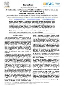
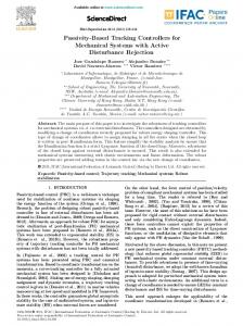
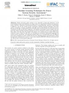
5. SOFTWARE IMPLEMENTATION Based on the reasoning of the previous section, the choice of the software framework is motivated and the software package casiopeia is introduced. 5.1 Choice of software framework A framework that satisfies the requirements formulated in Section 4.2 and with this facilitates the use of (18) for formulation and solution of (20) is casadi, introduced by Andersson (2013). It does so by providing the possibility to automatically generate derivative expressions using AD principles for complex symbolic expressions as well as for calls to external solvers that have been coupled to casadi in a way that supports AD. These expressions can be used to formulate and solve optimization problems, while all derivatives that are needed by the NLP solvers that interact with casadi are generated automatically. 5.2 Introduction of the software package casiopeia The implementation of the presented methods is included in the open-source Python module casiopeia (B¨ urger, 2016). In addition to PE and OED features, a collection of tools is provided in order to help the user to assess the quality of the estimation results. The implemented methods can be used via a unified user interface. Furthermore, multiple shooting and collocation discretizations for dynamic systems are generated automatically. A detailed documentation including introductory examples can be found in (B¨ urger, 2016). For the solve() command introduced in Section 3.1, the numerical linear solver csparse (Davis, 2006) is used, which is available as an infinitely many times differentiable function through casadi and is also able to exploit the sparsity structure of the involved matrices. 6. NUMERICAL CASE STUDY Within this section, the methods implemented in casiopeia are applied to a numerical example and their performance is assessed in terms of solution quality and computational effort. The code for the example can be found in (B¨ urger, 2016). 6.1 Model description The model used within this example describes the dynamics of a quarter vehicle, a system that is used in analysis of road performance and driving characteristics of vehicles. Within the model, a spring-damper-system depicts a vehicle’s chassis that is coupled to another spring that reflects the behavior of the tire. A schematic depiction of the system and a description of the symbols used within the model is given in Figure 1. The dynamics of the quarter vehicle can be described by a system of ordinary differential equations (Mitschke, 2014)

Symbol

Description

Unit

kC

Chassis damper coefficient

cC

Chassis spring coefficient

cT

Tire spring coefficient

Ns m N m N m

mC

Vehicle mass

kg

xC

Vehicle mass deflection

m

vC

Velocity in xC direction

m s

mT

Tire mass

kg

xT

Tire mass deflection

kg

vT

Velocity in xT direction

g

Gravitational acceleration

m s m s2

u

Deflection from ground

m

g

u ¯(t) = 0.05 m · sin(2πt).

mC xC cC

kC

These inputs are assumed to be subject to noise, so that the inputs that actually excite the system and therefore are used for simulation are

mT

u e=u ¯ + N (0, Σw )

xT cT u

Fig. 1. Schematic depiction of the quarter vehicle system model and description of symbols. x˙ T (t) = vT (t) kC cC v˙ T (t) = (vC (t) − vT (t)) + (xC (t) − xT (t)) mT mT cT (xT (t) − u(t)) − (21) mT x˙ C (t) = vC (t) kC cC v˙ C (t) = − (vC (t) − vT (t)) − (xC (t) − xT (t)). mC mC The system states x> = [xT , vT , xC , vC ] describe the positions of the involved masses and their current velocities. The parameters p> = [kC , cC , cT ] describe spring and damper coefficients to be determined experimentally. The input u describes the deflection of the tire bottom from the ground, which is either introduced by random road undulation during driving, or applied by an apparatus in order to run certain experiments for the system.

pinit

    1.0 · 103 Ns kC,init m    N . =  cC,init  =  1.0 · 104 m 

ptrue

Table 1. Comparison of parameter values and standard deviations, initial experiments. kC (103

Parameter

L−1

cT,true

1.6 ·

(22)

N 105 m

and all initial states x(t = 0) set to 0. Noise is applied to the generated simulation results as in ye = y¯ + N (0, Σy )

(23)

to reflect noisy measurements. In general, Σy is a blockdiagonal matrix with the (co-)variances of the measurements σy2 at each time point. For simplicity, we assume that the noise of the several measurements is uncorrelated here, such that σy only contains the diagonal entries   diag(σy ) = 0.01 m, 0.01 ms , 0.01 m, 0.01 ms .

PL i=1

i=1

As a result, Σy is also a diagonal matrix. The inputs u ¯ that are sent to the system are

pˆi

(ˆ pi − pˆmean

)2

pˆL

p

diag(βzˆL ΣpˆL )

Ns ) m

cC (104

N ) m

cT (105

N ) m

4.082

3.973

1.616

0.1245

0.1455

0.0264

4.141

3.965

1.650

0.1143

0.1284

0.0254

Table 1 shows that the estimated parameter values lie in the neighborhood of ptrue , but with comparatively high standard deviation, which is caused by the insufficient system excitation introduced by u ¯. Also note that the standard deviations computed by casiopeia are close to the standard deviations of the repeated experiments. 6.3 Optimum experimental design Based on the initial input trajectory u ¯ and using the estimated parameters pˆL from Section 6.2, optimized inputs u ˆ are obtained using the OED routine of casiopeia. Upper and lower bounds on the state values and the input values are introduced as follows    0.1 m 0.1 m m m  0.4 s  0.4 s  = − ,x = , 0.1 m  max 0.1 m m m 0.4 s 0.4 s 

xmin (24)

(27)

N 105 m

The scaled mean values pˆmean of all estimates pˆi and the corresponding standard deviations are then computed and compared to the result of the last estimation pˆL and the standard deviations obtained from the evaluation of βzˆL ΣpˆL in casiopeia. The results are shown in Table 1.

pˆmean = L

    kC,true 4.0 · 103 Ns m    N =  cC,true  =  4.0 · 104 m 

1.0 ·

cT,init

q

Sample data y¯ of all system states are obtained by simulation of (21) for a time horizon of tf = 5 s at a sampling rate of fs = 20 Hz with assumed true parameters

(26)

2 with Σw a diagonal matrix with entries σw = 0.0052 m2 . This input noise is a special kind of process noise. Following these steps, data are generated for L = 100 repeated estimations of pˆ with the PE routine of casiopeia. To compensate for the noise on u e, additional degrees of freedom w ∈ Rnw with nw = nu are introduced to the PE problem. Since the expected order of magnitude for the values in pˆ is assumed to be known, the parameters are scaled accordingly within the estimation. The initial guess for pˆ used within the estimation is

PL −1

6.2 Parameter estimation

(25)

umin = −0.05 m, umax = 0.05 m,

(28)

(29)

Initial inputs u¯

Tire bottom deflection (m)

0.06

Optimized inputs uˆ 103

Evaluation time (s)

0.04 0.02 0.00 −0.02 −0.04 −0.06

0

1

2

3

4

5

Time (s)

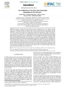
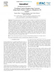
in order to generate experiments only within the system’s (assumed) operation range. As information function Φ the A-criterion, i. e. the trace of Σp , is used. Figure 2 shows the optimized inputs u ˆ in comparison to the initial inputs u ¯, depicting how the optimized inputs are used to intentionally excite different parts of the system and increase the information content. The increase in confidence achieved by the experimental design can be visualized by a comparison of the confidence ellipsoids that result from the initial and optimized inputs, which is shown in Figure 3 for parameters kC and cT . 6.4 Parameter estimation from optimized experiments Using u ˆ, optimized measurement data yˆ are generated according to Section 6.2 and the estimations are repeated with otherwise unchanged settings. The results are shown in Table 2. Table 2. Comparison of parameter values and standard deviations, optimized experiments. kC (103

PL −1

pˆmean = L

q

PL −1

L

i=1

i=1

pˆi

(ˆ pi − pˆmean )2

pˆL

p

diag(βzˆL ΣpˆL )

Ns ) m

cC (104

N ) m

cT (105

N ) m

4.027

3.985

1.604

0.0592

0.0784

0.0177

3.992

4.013

1.596

0.0559

0.0814

0.0172

Table 2 shows that it is now possible to retrieve confident estimates for all parameter values that lie very close to ptrue . This shows that not only more reliable estimates can be obtained based on the optimized experimental data, but also less experiments would be necessary in order to obtain this level of certainty. 4.160

Initial inputs u¯

Optimized inputs uˆ

kC (103 Ns m)

4.150 4.145 4.140 4.135 4.130 4.125 1.63

1.64

1.65

Schur complement (18)

2

101 100 10−1 10−2 2 10

103

104

1.66

1.67

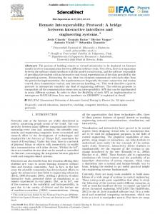
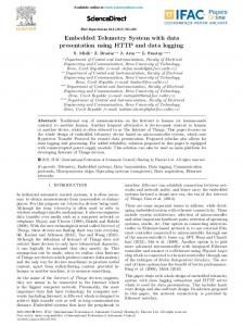
Fig. 4. Comparison of covariance matrix evaluation time on an Intel Core i5-4570 3.20 GHz CPU. In case further improvement was desired, the design and estimation procedures could be repeated based on the improved estimation results. Furthermore, casiopeia could be used to design multiple experiments within one optimization problem to obtain complementary experiments that deliberately excite different system parts. 6.5 Performance of the Schur complement method To assess the performance of the method in (18), Σpˆ is computed for different time horizons tf which result in a different number of discretization intervals. The computation times are compared to those of the other approaches shown in the previous sections, i. e., evaluating Σpˆ as in (5) for a single shooting implementation of the PE problem according to (1), to the direct evaluation of K −1 given in (10) and to the direct factorization approach in (15). To simplify the comparison, a fourth-order Runge-Kutta method with fixed step size is used for discretization of the dynamic systems. Figure 4 shows that the Schur complement method in (18) is the most efficient approach within this comparison. The evaluation time increases almost linearly with the number of discretization intervals N (which here is equivalent to an increase in measurements, see Section 2.1). The methods (5), (10) and (15) show a much more rapid increase in evaluation time. Missing entries in Figure 4 indicate that the evaluations either did non finish in reasonable time, or the limitations of approximately 14 GB of available memory were exceeded. 7. CONCLUSIONS AND FUTURE WORK Within this paper, a Schur complement method for OED has been presented that is particularly well suited for PE problems with process noise. The method has been implemented in the open-source software package casiopeia based on the symbolic framework casadi and tested on a numerical example.

4.155

4.120 1.62

Direct Factorization (15)

Single Shooting (5)

Number of discretization intervals N

Fig. 2. Comparison of initial and optimized inputs.

Parameter

10

Full inversion (10)

1.68

N cT (105 m )

Fig. 3. Comparison of confidence ellipsoid of parameters kC and cT for initial and optimized inputs.

While the advantages over other approaches have been investigated, it is subject to further research how the evaluation time can be further decreased to facilitate OED problems of larger size. Since the Schur complement approach to compute the covariance matrix is rather generic, the method can easily be extended to directly support other types of noise as well.

REFERENCES Andersson, J. (2013). A General-Purpose Software Framework for Dynamic Optimization. PhD thesis, Department of Electrical Engineering (ESAT/SCD) and Optimization in Engineering Center, KU Leuven. Annergren, M. (2016). Application-Oriented Input Design and Optimization Methods Involving ADMM. PhD thesis, KTH Royal Institute of Technology. Bauer, I., Bock, H.G., K¨ orkel, S., and Schl¨ oder, J.P. (2000). Numerical methods for optimum experimental design in DAE systems. Journal of Computational and Applied Mathematics, 120(1-2), 1–25. Bock, H.G. (1983). Recent advances in parameter identification techniques for ODE. In Numerical Treatment of Inverse Problems in Differential and Integral Equations, 95–121. Birkh¨ auser. Bock, H.G., K¨ orkel, S., Kostina, E., and Schl¨ oder, J.P. (2007). Robustness Aspects in Parameter Estimation, Optimal Design of Experiments and Optimal Control, 117–146. Springer Berlin Heidelberg, Berlin, Heidelberg. doi:10.1007/978-3-540-28396-6 6. URL http:// dx.doi.org/10.1007/978-3-540-28396-6_6. Bock, H.G., K¨ orkel, S., and Schl¨ oder, J.P. (2013). Parameter Estimation and Optimum Experimental Design for Differential Equation Models, 1–30. Springer, Berlin, Heidelberg. B¨ urger, A. (2016). casiopeia – Casadi Interface for Optimum experimental design and Parameter Estimation and Identification Applications. https://github.com/ adbuerger/casiopeia. Davis, T.A. (2006). Direct methods for sparse linear systems. Fundamentals of algorithms. SIAM, Society for Industrial and Applied Mathematics, Philadelphia. Golub, G. and Loan, C. (1996). Matrix Computations. Johns Hopkins University Press, Baltimore, 3rd edition. Griewank, A. (2000). Evaluating derivatives : principles and techniques of algorithmic differentiation. Frontiers in applied mathematics ; 19. SIAM, Philadelphia. K¨ orkel, S. (2002). Numerische Methoden f¨ ur Optimale Versuchsplanungsprobleme bei nichtlinearen DAEModellen. PhD thesis, Interdisciplinary Center for Scientific Computing, Heidelberg University. K¨ orkel, S., Kostina, E., Bock, H.G., and Schl¨ oder, J.P. (2004). Numerical methods for optimal control problems in design of robust optimal experiments for nonlinear dynamic processes. Optimization Methods and Software, 19(3-4), 327–338. Kostina, E. and Kostyukova, O. (2012). Computing Covariance Matrices for Constrained Nonlinear Large Scale Parameter Estimation Problems Using Krylov Subspace Methods, 197–212. Springer Basel, Basel. Ljung, L. (1999). System identification : theory for the user. Prentice-Hall information and system sciences series. Prentice Hall, Upper Saddle River, NJ [et al.], 2. edition. Mitschke, M. (2014). Dynamik der Kraftfahrzeuge. Springer Vieweg, Wiesbaden, 5. edition. Nocedal, J. and Wright, S.J. (2006). Numerical Optimization. Springer Series in Operations Research and Financial Engineering. Springer, 2 edition. Press, W.H. (ed.) (2007). Numerical recipes : the art of scientific computing. Cambridge University Press, Cambridge [et al.], 3. edition.

Pronzato, L. (2008). Optimal experimental design and some related control problems. Automatica, 44, 303– 325. Rao, C.V., Rawlings, J.B., and Mayne, D.Q. (2003). Constrained state estimation for nonlinear discrete-time systems: Stability and moving horizon approximations. IEEE Transactions on Automatic Control, 48(2), 246– 258. Walter, E. and Pronzato, L. (1997). Identification of parametric models from experimental data. Communications and control engineering. Springer [et al.], Berlin.