SCnC: Efficient Unification of Streaming with Dynamic Task Parallelism Dragos¸ Sbˆırlea
Jun Shirako
Ryan Newton†
Vivek Sarkar
Rice University, Indiana University†
[email protected] [email protected] [email protected] [email protected]
Abstract Stream processing is a special form of the dataflow execution model that offers extensive opportunities for optimization and automatic parallelization. To take full advantage of the paradigm, however, typically requires programmers to learn a new language and re-implement their applications. This work shows that it is possible to exploit streaming as a safe and automatic optimization of a more general dataflow-based model—one in which computation kernels are written in standard, general-purpose languages and organized as a coordination graph. We propose Streaming Concurrent Collections (SCnC), a streaming system that can efficiently run a subset of programs supported by Concurrent Collections (CnC). CnC is a general purpose parallel programming paradigm with a task-parallel look and feel but based on dataflow graph principles. Its expressivity extends to any arbitrary task graph. Integration of these models would allow application developers to benefit from the performance and tight memory footprint of stream parallelism for eligible subgraphs of their application. In this paper we formally define the requirements (streaming access patterns) needed for using SCnC, and outline a static decision procedure for identifying and processing eligible SCnC subgraphs. We present initial results on an prototype implementation that show that transitioning from general CnC to SCnC leads to a throughput increase of up to 40× for certain benchmarks, and also enable programs with large data sizes to execute in available memory for cases where CnC execution may run out of memory.
1.
Introduction
As multicore computing becomes the norm, rather than the exception, exploiting parallelism in applications becomes paramount. Parallel programming models based on stream processing are of particular interest because they offer some of the best examples of high-performance, fully automatic parallelization of implicitly parallel code. However, programming languages built around stream programming, such as StreamIt, have not become widespread, even for application areas where they offer clear benefits. This may be due to the intrinsic adoption barrier for new programming languages—especially those with a narrow range of applicability or which do not compose with larger software systems. We propose a new solution to this problem that can enable efficient stream processing within general applications written using standard languages (in this paper, Java). We do not, however, attempt to optimize streaming patterns within a fully general-purpose language. Rather, we advocate targeting stream-processing patterns implemented within a more general-purpose graph-based parallel model. To that end we target the Concurrent Collections model. Concurrent Collections (CnC) is unique in exposing a taskparallel “look and feel” while retaining determinism. CnC allows the user to dynamically launch tasks(“steps”) which read and write from single-assignment key-value stores (“collections”).
CnC is an effective parallel programming model for many problems. For streaming applications, however, it is rather inefficient, incurring task scheduler overhead and further overhead to store stream elements in heavy-weight geernal-purpose collections. In this paper we introduce Streaming CnC (SCnC), which identifies streaming patterns based on metadata already available in the CnC program. For compliant programs, SCnC uses an alternative code generation and runtime tool to enable improved performance and memory usage. We show the equivalence of the streaming and task-based execution of the same program and identify the additional restrictions needed to make streaming a safe optimization, insuring deadlock-freedom. The streaming CnC extension proposed is more general than many stream-parallel programming languages. We report ongoing work on the SCnC prototype implementation, including a performance comparison against the baseline CnC execution and expressiveness compared to the StreamIt. This paper offers the following main contributions: • The identification of a small number of restrictions to the CnC
language that allow the switch from a task-based to a streaming runtime while maintaining determinism and the representing a wider range of graph than the usual pipeline/split join / loopback streaming graphs. To our knowledge, no other streaming system supports this kind of streaming graph shapes. • An novel analysis to identify when a program is streaming (i.e.
will run correctly on the streaming runtime). • A new analysis to determine if the streaming execution is
deadlock-free even in the presence of variable input / output rates and to determine safe bound for the streaming buffers. • Experimental results showing compelling performance and
memory improvements compared to the task-based execution of the same application code.
2.
CnC Terminology
The Concurrent Collections(CnC) programming model [8] on which Streaming Concurrent Collection is a prerequisite to understanding the paper and is described in short in this section. CnC has three main building blocks: item collections, control collections and step collections. These collections and their relationships are defined statically for each application in a CnC textual graph specification file, but the code of the application, the step implementations, can be written in any one of multiple host languages. Step collections correspond to particular functions defined in the host language. A step instance is analogous to a task being spawned (or a streaming filter iteration). Where we would say a task has been spawned, we say a step instance has been prescribed. In contrast to streaming, the CnC model does not imply any ordering constraints between execution of step instances of the same step collection; however, steps read and write data which introduce dependencies (items). Steps are stateless and have no side effects
Edge type Item Put
Source Collection Step
Destination Collection Item
Control Put
Step
Control
Item Get
Item
Step
Prescription
Control
Step
Meaning
CnC application
a source step may put items in the destination item collection a source step instance may put control tags in the destination collection A destination stepmay get items from the source collection Any tag put in the source control collection leads to the execution of a step instance from the destination collection.
Table 1. Types of edges in a CnC graph outside of item production/consumption. The main program that initiates a CnC graph, provides its inputs, and reads its outputs is referred to as the environment for the CnC graph. Item collections are CnC’s data layer and accessing items is the sole means of synchronization between steps. Item collections are “append-only” key-value stores with the keys referred to as item tags. Any step collection that shares an edge with an item collection in the application graph can perform a Put or Get operation to access items in that collection, according to the direction of the edge. However, individual items are single-assignment and cannot be overwritten. Further, reading an unavailable item requires blocking until the item is provided by another step instance. With step collections for computation and item collections storing data, the final collection type, control collections, serve as broadcast nodes, sending invocation messages (also called control tags) to one or more step collections, prescribing an instance of each to execute. The only operation on control collections is thus a Put(controlTag) whose parameter is passed to the step instance as an argument. The CnC graph specification is a textual representation of the statically known structure of the application, relating the application’s step, item, and control collections, as well as including metadata about item tag indexing relationships (data access patterns). The graph is used to generate code for the item and control collections and to construct and execute the graph, so that the user need write only step implementations. For graphical representations in this paper, we use the following shapes, following standard CnC conventions: step collections are circles, item collections are squares and control collections are triangles. Table 2 shows the various types of edges forming a CnC application graph. To execute general CnC programs a task based runtime is needed. Currently, the runtime spawns task for each step instance, uses hashmaps to implement item collections and locks for synchronization on items. Dataflow programming models and indeed any programming model have to establish a compromise between expressiveness and analyzability [14]. CnC supports a wide range of application graphs and provably supports more parallel execution graphs than Cilk: while Cilk supports fully strict computations[4] that are also terminally strict [2], CnC can express any terminally strict computation [12].
3.
Streaming CnC
Streaming CnC (SCnC) provides a restricted version of the CnC model (including the graph specification, corresponding code generator, and runtime library) that allows efficient streaming execution of CnC programs, as opposed to task based execution used for non-streaming CnC applications. Ultimately, SCnC will execute
Convert graph to well formed shape (Section 8)
No
Success in converting?
No
Is the graph well formed?
Yes
Yes
Fail
Check streaming access pattern (Section9)
Ok Identify deadlock safety bounds (Section 10)
Map to task based runtime
Map to HJ & streaming phasers (Section 12)
Task based CnC application
Streaming CnC application
Figure 1. The high level algorithm needed to convert a CnC application to streaming form CnC applications using the same source code and specifications as CnC. (But our present prototype has minor API differences, described in Section 6.2.) A theoretical description of the SCnC subset of CnC application is presented in Section 3.1 and the engineering considerations behind our choice is presented in section 6. The process of running applications in the presence of CnC and SCnC is illustrated in Figure 1. As reflected in the Figure, our current prototype makes an all-or-nothing decision as to whether an application is streaming. However, there is no reason that SCnC sub-programs cannot execute alongside their CnC counterparts in the future. SCnC is based on a mapping between CnC and streaming concepts (as in Table 2). We identify a subset of CnC graphs where this mapping is valid and efficient which we call well-formed [for SCnC]. We show how analyze applications to test well-formedness of applications in Section 4. If the application data accesses are streaming, we identify buffer sizes that eliminate the possibility of deadlocks (Section 5). As a last step, mapping to the actual streaming runtime is performed, as discussed in Section 6. This paper compares the performance of running the same applications on the streaming and task-based runtimes. We also compare the performance of SCnC against StreamIt to identify how much of the streaming performance benefit we were capable of extracting automatically, while allowing the programmer to use a single, high level language for both streaming and non-streaming applications. 3.1
Streaming CnC graphs
The SCnC runtime cannot run an arbitrary CnC graph. This is because of the nature of streaming (not any application is a streaming application), because of implementation considerations, and because of language design restrictions (compromise between generality and safety guarantees such as determinism and deadlock freedom). We named this subset well-formed, defined as follows: Definition A well-formed SCnC graph is a CnC graph that respects the following conditions: 1. Control collections have only one producing step collection and one prescribed step collection. 2. Item collections have only one producing and one consuming step collections. 3. The environment only puts control tags into a single control collection and has no other put-edge. The control tags can be pairs that include the value of any items that for convenience, are produced by the environment.
CnC name Item collection Control collection Step collection Environment
Streaming name Queue between filters No exact match in streaming Filter Input stream
API SCnC collection.get(0)
collection.get(x), peek(y) with x > 0
Table 2. Mapping between CnC concepts and streaming concepts Definition The CnC control graph is the CnC graph with the item collections, item put-edges and item get-edges removed. T HEOREM 3.1. For a well formed CnC graph, the CnC control graph with root the entry control collection is a directed tree. Proof We first prove the absence of cycles. We know the CnC control graph is weakly connected and that both step and control collections have only one predecessor and can be reached from the environment. If there was a cycle, the nodes in that cycle would have a predecessor in the cycle, so either the environment is in the cycle (impossible, as the environment does not have any incoming edges) or the cycle is unreachable from the environment (impossible). Because it does not have cycles, the CnC control graph with entry control collection as root is a directed tree. We know that there is a path from the environment to each step collection . As the entry control collection is the singular child of the environment, all paths must pass through it, so there must be a path from the entry control collection to every node. We now check for the proper direction of the edges: control graph edges are either from control collections to step collections or from step collections to control collections. Each step collection has only one incoming edge (the prescription edge) witch connects the step collection to its parent in the tree, leaving the ether edges to connect the step collection to children.2 The SCnC runtime supports a large subset of general CnC applications, as long as the application has streaming access patterns for items, as defined in Section 4. SCnC introduces the separation of control streams (CnC control collections) and item streams(CnC item collections), where control streams are similar to the variables that guide the flow through the basic blocks of a control flow graph in program analysis. By Theorem 3.1 the CnC control graph of a SCnC program is a directed graph. Furthermore, any tree can be a CnC control graph; we can obtain the CnC control graph by expanding all of the directed tree nodes to a pair of control collection connected to a step collection and keeping all the original tree edges as edges from the step collection of the source to the control collection of the destination. On this directed tree backbone, adding any item stream with any single source and any single destination step collections keeps the result a legal CnC program. The generality of the supported graph shapes was a priority, and allows streaming a larger set of applications than other streaming frameworks. A comparison of the expressiveness of SCnC and other streaming languages, is in the Related Work section. 3.2
Streaming CnC vs. CnC vs. StreamIt
Some CnC concepts map naturally to streaming concepts: item collections seem like the streaming queues and steps look like filters. Of course, there are differences such as the explicit control flow in CnC and the formalization of the environment. The mapping between streaming constructs and SCnC constructs is in Table 2. SCnC restriction to single producer for item collections forces the distribution/duplication operations to be explicit in the SCnC graphs, which in turn helps solve the determinism problems that might arise in a multiple producer/consumer scenarios with implicit
Streaming pop()
Description remove and return the next element in the queue get(x) returns the element that has been popped by the x-th previous get(0) on that collection; peek(y) return the item at offset y in the queue
Table 3. Item get API: mapping between streaming and SCnC joins. Because in SCnC the join step explicitly states the order of the gets and puts from each of the input collections, based on the value of the control tag it receives from its control collection, determinism is maintained and this allows for arbitrary split/join patterns compared to StreamIt. The API of the item collection operations are similar to those on streaming queues, as Table 3 shows, with get(0) corresponding to a pop() operation. A get with a parameter different than 0 is similar to a ”reverse peek” operation that allows access to the element obtained M pop operations ago; using it, we can express any operation that can be expressed with a traditional peek. In many applications, one pattern that appears in the graph is the item collection - step collection cycle. This means that a single step collection is both producer and consumer of an item collection and for well-formed graph the step collection, being the single producer and consumer, is the single entity to interact with the item collection. We call such item collections step-local item collections. We have identified the cause of this pattern to be the restriction of CnC that the steps are stateless (that is, there is not state information preserved between different step instance executions). If the application access pattern is streaming, these collections can be transformed back to variables as state is permitted in SCnC.
4.
Streaming access pattern identification
SCnC only runs streaming programs; as the streaming runtime is more restricted than general CnC, additional checks have to be performed before using it. This section deals with the required checks for automatic identification of the streaming access patterns on a well-formed graph. In this section, we take the well-formed shape of the application graph as a given and use the theorems in section 3.1 to support our analysis. There is no corresponding transformation, just a boolean answer that ensures the application will run on the streaming runtime. The algorithm is a completely new and has two parts: graph analysis and condition testing. The testing phase can throw errors that mean the application does not respect the item restrictions that we define as streaming. In the following algorithm, any step that requires the computation of a function that cannot be identified (for example if the output value is not dependent only on the parameters specified) will fail and lead to early termination of the algorithm and output of FALSE (application cannot be converted to streaming form using simple rewrite rules). The functions that annotate edges in this algorithm are user written. The identification of functions and equation solving needed to make the analysis work can be implemented using symbolic execution methods, specifically symbolic evaluation, from systems such as Magma [6]. Such mathematical modeling has now made its way into commercial tools like Matlab [1]. In CnC applications these functions are typically not complicated, usually linear functions, which considerably simplifies analysis.
The analysis phase of the algorithm consists of these steps: 1. Require the control tags of the EntryStep ( the Env− > EntryT ags edge) to be consecutive integers starting from 0. These are iteration numbers and work like time steps.
function of each step with each of its item Get functions: S−I I S for example fconsumer = fitemGet ◦ fproducer gives the item consumer function for an item collection I consumed by step collection S.
2. Require all item and control tags of to have an integer ordering component, unique in the tags of the particular item or control collection. This ordering component and should be monotonously increasing. In the following steps of the algorithm for simplicity , we refer only to this ordering component as the tag, even though there may be other information used in the real tag.
5. For each item-put or item-get edge in the graph, compute the minimum consumer function, defined as the minimum of the values of all the consumer functionsfor a step instance. I fmin consumer (y) = minx (fcx (y)) The intuition is that they identify the smallest tag that a step can get from the item collection I, as a function of the time iterations used as entry control tags for the graph.
3. The following steps compute labels on the application graph that map control tags of producers or consumers to the item or control tags that get produced/consumed by that step:
Note that, according to Theorem 3.1 if there are item-put and item-get functions, the composition of the functions required for the existence of producer functionsand consumer functionsexists. The purpose of the test phase is to test the fact that the graph functions respect the streaming access restrictions to items. It consists of testing that the producer and consumer function pairs for all item collections respect the following constraints:
• Annotate each item put-edge between a step T and an item
collection O with at least one item put-function with domain equal to the possible control tags for step T and codomain equal to the tags of the items that are put. If a step instance can put k items, there have to be k distinct putfunctions, to model the relationship between the tag of the step and the possible tags of the items produced. If the number of item-puts a step instance can perform is not bounded, the algorithm fails. If the functions cannot be identified statically, for example when the item tags depend on the value of other data items, it also fails. • Annotate each control put-edge with similar control (tag) i put functions fcontrolP ut .
• Annotate each item get-edge with similar item get funci . tions fitemGet
• Label each prescription edge with the identity function
4. Compute meta-functions that map iteration numbers (entry control tags for the streaming graph) to item and control tag values that get produced by composing the previously defined functions. • Do a traversal of the CnC control graph(which is an arbores-
cence according to Theorem 3.1), labelling each step collection and item collections with the result of the composition of the functions through which the path from the root of the tree passes to reach that particular step. We call this label function a producer function for that step, control or item collection. For example, if the path from the EntryStep collection to a step collection S goes through the edges labeled, in order, with the control put functions f1 to fn , the producer funcS tionfor that control collection is: fcontrolP ut = fn ◦ fn−1 ◦ fn−2 ◦ ... ◦ f1 . If the step collection S produces items in the item collection I, and the item put edge between them is S−I labelled with item-put function fitemP ut , then the producer S−I I functionfor item collection I is: fproducer = fitemP ut ◦ S fcontrolP ut The traversal is easily done in a pre-order traversal, thus incurring only a linear complexity cost. For each item collection, there will result a set of producer functions, that map iteration numbers (tags coming from the environment) to item tags. The intuition behind these functions is that they give the item tags that are produced at a certain iteration.
1. “producer precedence” constraint: any item is produced in an earlier iteration that it is consumed. If fc and fp annotate edges that share a common item collection vertex and y is an item tag, then fp−1 (y) ≤ fc−1 (y), ∀y ≥ 0. If there is no inverse for either functions of any item collection or if the previous relationship simply does not hold, return FALSE. 2. “bounded buffer” constraint: there is a constant N1 such that for any pair of consumer functions fc1 and fc2 of a step collection, the difference between the value of the consumer functions is smaller than N1 . A step that respects this constraint will never consume items that are more than N1 items apart. The corresponding equation is: |(fc1 − fc2 )(x)| < N, ∀x and ∀fc1 and fc2 consumer functions of a single step collection 3. “sliding window” constraint: For a single step collection and consecutive step instances tagged y and y+1, the minimum value of the tag that can be consumed by the step tagged y+1 is no lower than the minimum value that can be consumed by step instance tagged y: fcmin (y) ≤ fcmin (y + 1) 4. “bounded lifetime” constraint: For any item tagged t, produced in iteration t1 and consumed in iteration t2 , there is N2 constant such that t2 − t1 < N2 Bounded buffer, sliding window and bounded lifetime assure that we will not need a buffer size larger than N1 or N2 to satisfy get calls on an item collection. 5. “unique timestep” constraint: Each step instance performs no more than a single put in each of its output control collections. This constrain assures us that, for a given step collection there will never be more than one step instance with the same iteration number (started by a single ancestor). If the functions of all item collections respect the previous constraint, then the algorithm outputs TRUE. Otherwise it outputs FALSE.
5.
Deadlock
SCnC must not introduce deadlocks to correct CnC programs. There are three possible causes of deadlock in SCnC, as follows: • If a step blocks attempting to get an item that cannot be pro-
duced because it requires the current step to complete (filter iteration ordering constraint). We show this cannot happen with SCnC.
• In addition to creating a function representing all item in-
• If a step performs a get on an item that is no longer in the
stances produced in an iteration, we create a similar function for all items consumed. That is, we compose the producer
streaming buffer (streaming access pattern constraint). We show this cannot happen with SCnC.
• The full-empty buffer problem [15, 20].Lets say one of the
streaming buffer queues (called A) becomes full, blocking the producer and thus prevents him from producing items in another queue (B). If the consumer will block too waiting on B because of this (and cannot unblock A), then there is a deadlock. We describe a technique that finds a sufficiently large bound for the streaming buffers so that they never fill up. The first scenario is a direct contradiction of the “producer precedence” rule. If the item is unavailable, its producer must not be able to run until a later iteration (counted by global “ticks” from the environment). But, by the “producer precedence” rule an item’s consumption sites must happen at the same or later iteration than the item was produced. We must take some care with the situation where production and consumption of an item fall in the same iteration. In this case both the consuming and producing step instances will begin execution during the iteration in question. To deadlock, they each would have to wait for an item produced by the other one, which means both of them block on get calls followed at some point by put calls that would unblock the other one. This situation, however, would deadlock in a normal CnC execution, contradicting our assumption that the program is correct under a regular CnC execution. The second scenario occurs only if the buffer size selected is too small, which is prevented by the upper-bound determination method described in the next section. Finally, the full-empty buffer problem has been previously studied in the literature [15, 20] and is characteristic of any streaming application with filtering capabilities. Previously proposed deadlock avoidance algorithms can be applied to SCnC applications.
collection (“unique timestamp” rule). The maximum number of tags that need storage is thus M = it2 − it1 but this limit applies for all control collections on the path between the producer and consumer steps. As for the item buffer size, we need to consider all pairs it1 and it2 that can produce, respectively consume any item tagged t and take the maximum of the different M values obtained. The combination of using sufficiently large buffers for item collections (L) and control buffers (M) leads to the deadlock freedom property of a SCnC program.
6.
Implementation
Here we describe our prototype implementation of SCnC, which currently has certain restrictions. Only complete programs are handled by SCnC (not yet subsets of CnC programs), and some phases must be performed by hand, notably converting to use the slightly different put and get API described in previous sections. The programmer workflow for SCnC usage is in Figure 2. 6.1
Habanero Java
The step code of SCnC programs and the SCnC runtime system itself are written using Habanero Java (HJ), a language derived from X10 which offers primitives for productive and easy to use parallel programming. The basis for parallel programming are asynchronously forked tasks called asyncs, which are synchronized by an enclosing finish block. Habanero Java supports a superset of the Cilk [5] spawn-sync parallelism; it eliminates the Cilk requirement that parallel computations should be fully strict(in HJ, join edges don’t have to go to the parent in the spawn tree) [? ]. For producer consumer synchronization we use phasers. Phasers [23] 5.1 Sizing Item Collection Stream Buffers are synchronization constructs that offer scalable synchronization between a dynamically variable number of tasks The phaser regisThe third bullet in the list of deadlock causes needs attentive analtration mode models the type of synchronization required: signalysis. This subsection describes how to statically identify a safe size only and wait-only modes for producer consumer and signal-wait of the streaming buffers such that this full-empty buffer deadlock for barrier synchronization. In our work, we use the producercan never manifest. First, it is important to notice that a program consumer form of synchronization. having only Control and Step Collections cannot deadlock, as the Phaser accumulators [22] are a reduction construct built over the control graph is always a tree. synchronization capabilities of Habanero phasers. Each producer For an item with tag t produced with the restrictions of a well(which is registered in signal mode) sends a value to be reduced formed CnC application we have the following equation: t = i j and then, when all producers have signaled to the phaser , the fproducer (it1 ) = fconsumer (it2 ) illustrating that the item was consumer (which is registered in wait mode) can be unblocked and produced in time iteration it1 and consumed in time iteration it2 . use the reduced value. An accumulator is associated with a phaser If there are multiple possible consumer functions, all combinations and needs to know the type of the values it is reducing (e.g. int) must be considered and the final buffer size should be the maximum and what is the reduction operation (e.g. SUM). The producers can of those identified through the following computation. The required buffer size for item t is (it2 −it1 )∗maxt=it1 ..it2 P OR(t),send their values and then signal the phaser. The producer’s will proceed after all signals have been received and it can access the where POR(it) is the producer output in iteration it. reduced value through the accumulator result call. The item rate is upperbound by a limit R, where R is less than An extension of the accumulators and phasers for streaming, the cardinality of the set of put functions corresponding to the called streaming phasers or phaser beams, improves the use of producer and item collection. these constructs for streaming programs by adding support for Also, there is an integer constant k fixed such that t2 − t1 < k bounded-buffer synchronization in phasers and accumulators. For which means that the items consumed by a step are produced a fixed phasers, the producer can signal at most k times more than the number of time-steps before(“bounded lifetime” constraint). Note consumer waited. Accumulator now contain an internal circular that the it2 − it1 difference is always positive , as per “producer buffer whose size reflects the bound k that is used to store the precedence” rule. additional items before they are consumed. Access to previously The item collection buffer size is thus upper-bound by L = consumed elements is permitted, within the limits of the internal (it2 −it1 )∗R = k∗R. If the actual buffer size of the item collection buffer, by providing an additional offset parameter to the result call. buffer is larger than L, the buffer will never fill, thus the producer This feature underlies the SCnC reverse peek operation. and consumer edges cannot participate in a deadlock cycle. This condition is not enough though, as, even though there is 6.2 Mapping SCnC onto Habanero Java space in the item buffer, there might not be space in the control collection buffers somewhere on the path between the producer and The implementation of streaming item and control collections is based on phaser accumulators for poarallelism between step colthe consumer (as shown previously, the control graph is a tree, so lections. For data-parallelism within a step collection we also use there is only one such path). To find an upper-bound for the size dynamic split-join nodes that split the step instances into a userof the buffers on this path, we should consider that each step can controllable, stateful number of tasks. produce at most one control tag per iteration per destination control
Listing 1. Item collection implementation code fragment public abstract class ObjectItemColection { p u b l i c p h a s e r ph ; public accumulator a ; p u b l i c O b j e c t Get ( i n t no ) { Object value = null ; i f ( no == 0 ) { ph . doWait ( ) ; value = a . objResult ( ) ; } else {...} return value ; } public void Put ( Object p ) { a . send ( p ) ; ph . s i g n a l ( ) ; }}
Listing 2. Code fragment of the abstract base class for a step public void s t a r t ( WrappedInt ta g ) { f i n a l Tag f t a g = t a g ; async phased ( p C o n t r o l C . ph, / / p r e s c r i b i n g c o l l e c t i o n p r o d u c e d I t e m C 1 . ph , p r o d u c e d C o n t r o l C 1 . ph ) { run ( f t a g ) ; }} public void run ( WrappedInt ptag ) { W r a p p e d I n t t a g = c o n t r o l C . Get ( 0 ) ; while ( t a g . v a l u e != endStream ) { s t e p ( t a g ) ; / / run t h e u s e r w r i t t e n s t e p code t a g = c o n t r o l C . Get ( 0 ) ; / / pop t h e n e x t c o n t r o l t a g }}
Each collection has a phaser and accumulator pair that allow synchronization and communication between the producer and consumer of an item collection. The SCnC code generator creates a class with these two members and corresponding put and get operations. There are separate classes for primitive types for performance reasons and a specialized class for the actual type of the data items is generated by inheritance and performs the necessary type-casting from Object to the particular item type. Populating the EntryTag control collection with initial values is done through the init function in which the user adds code with Put operations. We generate both the graph class and the main program for the CnC application, which can be modified by the user, so the user only writes the step code. The difference in API compared to CnC is in put and get operations. Put operations always put the next item in the item collection (stream) and get operations take as input, not an absolute tag, but an offset relative to the position of the item produced by the last wait operation on the phaser of the item collection. Thus, the API for an item get operation are: if the desire is to access an already used item (an item that has already been gotten at least once), use get with an offset larger than 0. If the intent is to access the next item in the stream, then do a get with parameter 0, which means for the runtime that a new item has to be obtained and it inserts the proper wait operation on the item collection phaser. The essential operations of the functions are found in Listing 1. As described above, the phaser synchronization construct needs to be registered on the task that uses it. In our Habanero Java implementation, step collections are modeled through asyncs containing a loop, whose iterations correspond to step instances. The implementation is hidden from the user through auto-generated code and using object oriented class hierarchy. The translator creates a base abstract class for each step collection and the template for the actual user step class. The user only works with the user step class, in which he inserts code in only one function, as shown in Listing 2.
Figure 2. The tool workflow for streaming a CnC app. Blocks marked with a star are manual, in the current implementation.
7.
Experimental Results
The SCnC translator and runtime have been tested on a total of six applications: three StreamIt benchmarks (BeamFormer, FilterBank and FMRadio), a clustering application (FacilityLocation), the well known mathematical algorithm Sieve of Eratosthenes and a video processing application (EdgeDetection). Throughput results are shown in Table 4 for four of the applications; because of space constraints, the other benchamrks show only the additional speedup brought by exploiting dynamic parallelism (“SCnC dynamic” with dynamic split-join nodes), compared to an execution that fixes at compile-time the amount of data-parallelism exploited by a splitjoin construct (fixed graph). Results are reported for CnC, hand optimized phaser beams, and SCnC versions of the application. The work stealing scheduler of CnC has also been shown to perform well against other taskparallel implementations [10], and yet here we see a large opportunity for improved performance on streaming applications. Applications were initially implemented in CnC. Porting to SCnC by hand helped to validate our algorithm for transforming a CnC spec to SCnC. In this evaluation, we performed the analysis by hand and we manually refactored step code as well: first, changing Puts and Gets use the SCnC tags (offets rather than absolute time iterations), and, second, promoting step-local item collections to normal mutable state. The test results have been encouraging, with increases in throughput of up to 40x. In addition, SCnC showed it can support larger problem sizes than CnC due to memory footprint. The input sizes listed for CnC are the largest supported (given a 2GB Java heap). The SCnC results show the throughput for the same input size as CnC, but also for higher input size that is enabled by using SCnC. The tests have been performed on a system with four quadcore Xeon processors and 16GB RAM . The performance analysis focuses on the variation of throughput between implementations and not on absolute timing of applications, as the current CnC implementation has memory collection problems that lead to OutOfMemory exceptions for long running programs such as streaming ones [7]. The size of the problem used for CnC is the maximum size for which the garbage collection does not go over 10% of application runtime. One thread per core is used for the CnC runtime, which is based on a global work queue, whereas the streaming program instead employs one thread per node in the application graph (step). Therefore graph topology, and in particular the splitting factor at data-parallel split-join nodes, can have an impact on performance.
FMRadio Beamform Filterbank Facility Location
Input size (elements) 50,000 50,000 5,000,000 5,000,000 30,000 30,000 3,000,000 3,000,000 100,000 100,000 1,000,000 1,000,000 300,000 300,000 3,000,000 3,000,000
Model CnC SCnC SCnC Stream phasers CnC SCnC SCnC Stream phasers CnC SCnC SCnC Stream phasers CnC SCnC SCnC Stream phasers
Run Time (seconds) 44 9 400 34 60 7.8 140 51 102 3.4 29 5 54 13.2 150 65
Throughput (items/second) 1136 5555 12500 147058 500 3846 20270 58823 980 29411 34482 200000 5454 22727 20000 46154
Variant Variant M=N M=2*N
Execution Time (seconds) Consumer Delay SCnC SCnC dynamic none 90 94 1ms every 50th 212 101 1ms every 25th 414 131 1ms every 12th 857 250
Speedup 0.95 2.1 3.16 3.4
Table 5. Facility Location: Speedup using dynamic parallelism feature comapred with fixed parallel SCnC baseline, 16 core Xeon
The experimental results were performed according to the methodology suggested by Georges et al. [11]. 7.1
Benchmarks with fixed graph structure
This section addresses benchmark behavior under a compile-time determination of splitting degree for split-join nodes: i.e. a fixed graph structure. The FilterBank StreamIt application implements a filter bank for signal processing. The Beamformer version we implemented has deterministic output ordering and four parallel beams, as in the StreamIt implementation. 7.2
Dynamic parallelism benchmarks
The facility location application is a data mining application that solves the problem of optimum placement of production and supply facilities. Formally [16], we are given a metric space and a facility cost for each node as well as a stream of demand points. The problem is finding the minimum number and positioning of nodes such that it minimizes a cost function. This problem occurs in placing production facilities, networking and classification. In such a producer/consumer example, speedup by running multiple consumers in parallel is not possible, as they would block waiting for input to consume. We modeled the computation of such statistics by adding artificial wait times for consumers, starting from 0 to 1ms for every 12th point. The additional time is small, but it is enough to show some scalability of the parallel implementation of FacilityLocation. Higher values might correspond better to real world implementation but we decided to be conservative in our analysis, using at most 83.(3) microseconds per point. The results in Table 5 and show an additional speedup of 3.4 compared to a “fixed” parallel implementation.
Speedup Speedup 5.95 10.78
Table 6. Sieve: Comparison of SCnC performance with and without dynamic parallelism on the 16 core Xeon system, N= 1,000,000
A
Environment
B
Environment
Environment
C
Generator Frame Extractor
Frame Extractor
Input Frames
Input Frames
PrimeOwner ItemCollection
No. edges Edge Detector
DetectedEdes
Table 4. Performance results for StreamIt benchmarks (Filterbank, Beamformer, FMRadio) and FacilityLocation (16 core Xeon)
Execution Time (seconds) SCnC SCnC Dynamic 238 40 863 80
Count edges
No. edges Detector 0 Detector 30 Detector 60 Detector 90 DetectedEdes Count edges
Prime Filter
Prime Filter
PrimeSelector ItemCollection
Prime Filter
Distributor
Figure 3. A: the static CnC graph of EdgeDetection. B: the dynamic behavior of SCnC, using 4 parallel places. C: the dynamic behavior of Sieve, with 3 places.
The Sieve of Eratosthenes is an algorithm for finding the prime numbers, attributed to the Greek mathematician Eratosthenes. Our implementation (Figure 3) uses a dynamic split-join with feedback loop. There is one producer that streams in consecutive numbers starting at 2; the numbers are then sent to several parallel filters that check if the number is divisible with any of the prime numbers that each filter stores. If a filter finds a divisor, it sends to the join node a 1, if not, it sends 0. The join node performs a sum reduction and if the result is 0, the number is prime. It then sends back to the filters the id of the filter that should add the newly discovered prime number to its prime number store. Here the number of branches of the dynamic splitter can be adjusted to the number of cores in the machine. Each place stores a chunk of the primes previously found. Performance results are found in Table 6 for 15 filters and a cyclic distribution of primes to filters. We also implemented an extension of the Sieve that not only finds the prime numbers up to N, but also counts the numbers between N and M that are not divisible by any prime number less than N. With it we analyze the speedup of the split-join pattern without the overhead of variable granularity and added feedback synchronization as shown in Table 6. Our implementation of image edge detection application [9, 18, 19]: detectors rotate the image a certain angle and then apply a one dimensional convolution kernel. Because the convolution detects edges on a single dimension, the image is rotated to different degrees, edges are detected, the image is rotated back. Then, a join overlaps the result of the detectors and sums the pixels. This number is used to increase or decrease the number of detectors (angles) we will use for the next frame, to improve accuracy. The sum is sent through a loopback to the dynamic splitter which adjusts the number of detectors accordingly, as shown in Figure 7.2. For results, the number of edge detection filters was fixed to 2 ,4 and 8), although in practice it varies frame to frame, so that we can analyze the relationship between performance and the number of cores used. The relatively small speedup of SCnC compared to CnC for this application comes from the relatively small number of streaming operations performed: because the granularity of the tasks is higher (each iteration processes an full input image frame),
No. Detector Filters 2 4 8
Throughput (items/second Streaming phasers SCnC CnC 14.3 14.3 15.8 2.63 2.38 1.88 1.25 1.15 0.61
Table 7. EdgeDetection on the 16 core Xeon system the time consumed by the communication and synchronization, be it for a task-based or streaming runtime, pales in comparison.
8.
Related Work
The Lime project[3] allows loopback streams but only to destinations upstream from the source, disallowing streams to filters that are not on the path from the source to the root (input node) of the streaming graph. The stereo MP3 decoder described in Task Transaction Level Interface (TTL) system [13], is yet another example of streaming graph that cannot be represented using StreamIt easily. Because sinks consume streams from both sources, it is difficult to transform this shape to a hierarchical split-join one. The authors of the TTL paper focus more on the embedded implementation with limited resources and on reconfiguration and less on performance improvement due to streaming. No performance numbers and no comparison results are shown and the system is limited to streaming only. A comparison between the task-based dataflow model and streaming is started in [17], but their work relies on special language and the comparison with data-flow can only be taken as a guideline, as their dataflow implementation is not tweaked for performance, relying on the general Cilk model for short-lived tasks. The use of a single and synthetic benchmark, their use of different input language representations for the benchmark differentiate out work. Furthermore the results for the benchmark they propose are not entirely positive for their system. We show that consistently better results are possible for a larger number of real applications, even without using a custom-built streaming language, compiler and intermediate representation and while keeping the claim for determinism. Furthermore, we start from a dataflow language whose task-based implementation offers proved performance [10]. The closest work to our approach towards automatic streaming of task based programs is through extensions to OpenMP [21], but the OpenMP annotations, even though simple, are not easy to automatically infer and the generality of streaming graphs that can be expressed is limited by the use of OpenMP as foundation. Furthermore, the resulting program is not deadlock-free.
9.
Conclusion and future work
We have introduced a streaming model that enlarges the category of application graphs that can be considered streaming, compared with previous projects. We identified the constraints that an application should respect in order to adhere to the streaming model and proposed algorithmic analyses to check for these conditions, including deadlock avoidance. Complete implementation of this work would make streaming a safe and automatic optimization of general CnC programs. We showed the model offers significant performance improvement compared to the previous task-based approach of running such applications, with our without the dynamic streaming parallelism extension that we introduced through stateful places. Future work will consist of implementation of the analysis described in this paper and integrating SCnC with the task-based CnC runtime, so that the system can choose the streaming or task-based executions without any outside help. Our technique for dynamic
parallelism has a natural extension in dynamic pipelines where the Sieve results showed that even better speedups are possible.
References [1] MathWorks Symbolic Math Toolbox Documentation. URL www.mathworks.com/help/toolbox/symbolic/f1-82523.html. [2] S. Agarwal, R. Barik, D. Bonachea, V. Sarkar, R. K. Shyamasundar, and K. Yelick. Deadlock-free scheduling of x10 computations with bounded resources. SPAA ’07, New York, NY, USA. ACM. [3] J. Auerbach, D. F. Bacon, P. Cheng, and R. Rabbah. Lime: a javacompatible and synthesizable language for heterogeneous architectures. OOPSLA ’10, pages 89–108, New York, NY, USA. ACM. [4] R. D. Blumofe and C. E. Leiserson. Scheduling multithreaded computations by work stealing. J. ACM, 46:720–748, September 1999. [5] R. D. Blumofe, C. F. Joerg, B. C. Kuszmaul, C. E. Leiserson, K. H. Randall, and Y. Zhou. Cilk: an efficient multithreaded runtime system. PPOPP ’95, pages 207–216, New York, NY, USA. ACM. [6] W. Bosma, J. Cannon, and C. Playoust. The magma algebra system i: the user language. J. Symb. Comput., 24:235–265, October 1997. [7] Z. Budimlic, A. M. Chandramowlishwaran, K. Knobe, G. N. Lowney, V. Sarkar, and L. Treggiari. Declarative aspects of memory management in the concurrent collections parallel programming model. DAMP ’09, pages 47–58, New York, NY, USA. ACM. [8] Z. Budimlic, M. Burke, V. Cav´e, K. Knobe, G. Lowney, R. Newton, J. Palsberg, D. M. Peixotto, V. Sarkar, F. Schlimbach, and S. Tasirlar. Concurrent collections. Scientific Programming, 18(3-4), 2010. [9] J. Canny. A computational approach to edge detection. IEEE Trans. Pattern Anal. Mach. Intell., 8:679–698, November 1986. [10] A. Chandramowlishwaran, K. Knobe, and R. Vuduc. Performance evaluation of concurrent collections on high-performance multicore computing systems. IPDPS, pages 1 –12, april 2010. [11] A. Georges, D. Buytaert, and L. Eeckhout. Statistically rigorous java performance evaluation. OOPSLA’07, pages 57–76. ACM. [12] Y. Guo, R. Barik, R. Raman, and V. Sarkar. Work-first and help-first scheduling policies for async-finish task parallelism. IPDPS’09. [13] T. Henriksson, J. Kang, and P. van der Wolf. Implementation of dynamic streaming applications on heterogeneous multi-processor architectures. CODES+ISSS ’05, New York, NY, USA. ACM. [14] E. A. Lee. Balancing expressiveness and analyzability in stream formalisms, July 2008. [15] P. Li, K. Agrawal, J. Buhler, and R. D. Chamberlain. Deadlock avoidance for streaming computations with filtering. SPAA ’10, pages 243–252, New York, NY, USA. ACM. [16] A. Meyerson. Online facility location. FOCS ’01, pages 426–, Washington, DC, USA. IEEE Computer Society. [17] C. Miranda, A. Pop, P. Dumont, A. Cohen, and M. Duranton. Erbium: a deterministic, concurrent intermediate representation to map dataflow tasks to scalable, persistent streaming processes. CASES ’10, pages 11–20, New York, NY, USA. ACM. [18] M. Nijhuis. A Framework for Parallel Streaming Applications. Ph.D. dissertation, 2007. URL dare.ubvu.vu.nl/bitstream/1871/16168/1/dissertation.pdf. [19] M. Nijhuis, H. Bos, and H. E. Bal. A component-based coordination language for efficient reconfigurable streaming applications. ICPP ’07, Washington, DC, USA. IEEE Computer Society. [20] L. Peng, A. Kunal, B. Jeremy, C. Roger D., and L. Joseph M. Deadlock-avoidance for streaming applications with split-join structure: Two case studies. In ASAP, pages 333–336, 2010. [21] A. Pop and A. Cohen. A stream-computing extension to openmp. HiPEAC ’11, pages 5–14, New York, NY, USA. ACM. [22] J. Shirako, D. M. Peixotto, V. Sarkar, and W. N. Scherer. Phaser accumulators: A new reduction construct. IPDPS 09, . [23] J. Shirako, D. M. Peixotto, V. Sarkar, and W. N. Scherer. Phasers: a unified deadlock-free construct for collective and point-to-point synchronization. ICS ’08, pages 277–288, New York, NY, USA, . ACM.