Seabed classification from acoustic profiling data using the similarity ...

Seabed classification from acoustic profiling data using the similarity index Han-Joon Kim, Jae-Kyeong Chang, Hyeong-Tae Jou, Gun-Tae Park, and Bong-Chool Suk Korea Ocean R & D Institute, Ansan, P.O. Box 29, 425-600, Korea

Ki Young Kim Department of Geophysics, Kangwon National University, 200-701, Korea

共Received 22 January 2001; revised 19 October 2001; accepted 13 November 2001兲 We introduce the similarity index 共SI兲 for the classification of the sea floor from acoustic profiling data. The essential part of our approach is the singular value decomposition of the data to extract a signal coherent trace-to-trace using the Karhunen–Loeve transform. SI is defined as the percentage of the energy of the coherent part contained in the bottom return signals. Important aspects of SI are that it is easily computed and that it represents the textural roughness of the sea floor as a function of grain size, hardness, and a degree of sediment sorting. In a real data example, we classified a section of the sea floor off Cheju Island south of the Korean Peninsula and compared the result with the sedimentology defined from direct sediment sampling and side scan sonar records. The comparison shows that SI can efficiently discriminate the bottom properties by delineating sediment-type boundaries and transition zones in more detail. Therefore, we propose that SI is an effective parameter for geoacoustic modeling. © 2002 Acoustical Society of America. 关DOI: 10.1121/1.1433812兴 PACS numbers: 43.30.Ma, 43.30.Gv 关DLB兴

I. INTRODUCTION

includes a verification by dense sediment sampling and side scan sonar records.

High-resolution profiling systems are used to reveal geological structure of the sea floor composed of various types of sediments and rocks. A great deal of work has been performed to quantitatively determine or discriminate physical properties of the sea floor from profiling data. These studies encompass a wide spectrum of data processing. Earlier studies used monochromatic sonar data for the direct measurement of a pressure reflection coefficient of the sea floor.1 Milligan et al.2 introduced a statistical approach using the Karhunen–Loeve 共KL兲 transform. Instead of measuring the reflection coefficient, they utilized the entire acoustic echo signal from the sea floor. They classified the sea floor in a certain area according to the textural difference resulting from the cluster analysis of a whole set of data. With the development of a wideband chirp sonar, more quantitative approaches were introduced to estimate parameters of surficial sediments such as reflection and attenuation coefficients.3–5 The wide frequency band nature of the chirp sonar was also utilized to recognize the statistical properties of the bottom type based on time-frequency analysis.6 In this paper, we present the similarity index 共SI兲 as a new acoustic measure for sea floor classification. Our method is similar to that of Milligan et al.2 in that both are based on the KL transform. However, the computation of SI does not require the whole set of data like their cluster analysis does; instead, it is computed from several consecutive return traces. Further, SI, although computed statistically, is a physical parameter that appears to represent the variation of the sea floor in terms of surface texture and sediment type. Our discussions are illustrated with a real data example that 794

J. Acoust. Soc. Am. 111 (2), February 2002

II. THE SIMILARITY INDEX „SI… FROM THE KL TRANSFORM

The KL transform produces a set of uncorrelated 共orthogonal兲 principal components from the data set, thus has been widely applied to seismic data analysis and digital image enhancement.7–9 Although there are many ways to implement the KL transform, the singular value decomposition 共SVD兲 approach of Freire and Ulrych10 is a straightforward way. Let X be an acoustic profiling data matrix which contains M traces each with N data points, i.e., X⫽ 兵 x i j 其 ,

i⫽1,2, . . . ,M ;

j⫽1,2, . . . ,N.

共1兲

The SVD of X is given by r

X⫽

兺 ␴ i u i v Ti ,

i⫽1

共2兲

where superscript T indicates transpose, r is the rank of X, u i is the ith eigenvector of XXT, v i is the ith eigenvector of XTX, and ␴ i is the ith singular value of X. The singular values ␴ i are the positive square roots of the eigenvalues of the covariance matrices XXT or XTX 共Lanczos11兲. In Eq. 共2兲 the factor u i v Ti is an (M ⫻N) matrix of unit norm which is called the ith eigenimage of X. Since the singular values are always ordered in decreasing magnitude, the greatest contributions in the representation of X are contained in the first eigenimages. If the data are considered to be composed of traces which show a high degree of trace-to-trace correlation, X

0001-4966/2002/111(2)/794/6/$19.00

© 2002 Acoustical Society of America

may be reconstructed from only the first few eigenimages. Reconstruction using the first few singular values is called the principal component reconstruction. Whereas, reconstruction using the remaining singular values is called the misfit reconstruction. Freire and Ulrych10 showed that the percentage of energy contained in a reconstructed image is given by E, where

E⫽

q 兺 i⫽p ␴ 2i r 兺 i⫽p ␴ 2i

,

1⭐p⭐q⭐r.

共3兲

The choice of p and q depends on the relative magnitudes of the singular values, which are a function of the input data. The acoustic return from the sea floor is the sum of both reflected and scattered signals. In general, acoustic profiling data are gathered continuously in the form of signal traces at a very short interval. When the sea floor is flat over a short distance, we regard it appropriate that the sea floor condition varies negligibly, and consequently reflections are coherent. Whereas, the incoherent part of the data is assumed to arise from various inhomogeneities on a variety of scales at the sea floor and in its surficial volume that are reflective of roughness and degree of sediment sorting. There is a strong correlation between grain size and sorting;12 finer grained sediments are well sorted; in contrast, coarser grained sediments tend to be poorly sorted not only because they are hardly uniform in size but also because abundant intergranular pores accommodate smaller particles such as silt and fine sand. Coarse sediments will also increase the textural roughness of the sea floor. Therefore, coarse sediments increase inhomogeneities internal and external. These inhomogeneities are small compared with the wavelength of a pulse generated from acoustic profiling devices, giving rise to scattering. Milligan et al.2 showed that in their experiment the largest characteristic root of the covariance matrix accounted for 97% of the observed variance. This means that almost all of pure reflectivity of the bottom can be reconstructed from the first principal component. Although the analysis of Milligan et al. required all the acoustic return signals collected in the survey area, the same principle can be applied to a much smaller data set. If a coherent signal in adjoining traces refers to an event which is similar horizontally in a trace-to-trace sense, it is contained in the first eigenimage. We thus take q as 1 in Eq. 共3兲 to measure the coherence of a few consecutive return pulses. The resultant quantity is referred to as the similarity index 共SI兲:

SI⫽

␴ 21 r 兺 i⫽p ␴ 2i

.

共4兲

From Eq. 共4兲 it is easily conceived that SI ranges from 0 to 1 for various seabed conditions and increases in accordance with homogeneity and softness of the bottom. On the contrary, textural inhomogeneity and large roughness will result in a decreased SI value. J. Acoust. Soc. Am., Vol. 111, No. 2, February 2002

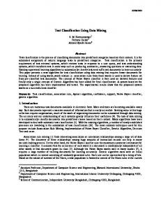
FIG. 1. 共a兲 Location map of the study area. 共b兲 Locations of chirp sonar profiles off the east coast of Cheju Island with positions of sediment sampling using a grab and by divers.

For some discrimination methods of the sea floor using acoustic profiling data, it is necessary to correct for amplifier gains and spreading losses. This is especially true when a pressure reflection coefficient of the bottom is directly measured. Even the statistical grouping method of Milligan et al.2 needed such correction to obtain mean acoustic reflection. The KL transform dictates that if X consists of M traces equal to within a scale factor, X can be perfectly reconstructed by the first eigenimage ␴ 1 u 1 v T1 . Therefore, SI is independent of ping-to-ping amplitude variation induced by extraneous factors such as amplifier gains and spreading losses. III. EXPERIMENT AND RESULT A. Data collection

A high-resolution profiling survey was carried out off the east coast of Cheju Island south of the Korean Peninsula 共Fig. 1兲. The chirp sonar system 共model: Data Sonics CAP 6000W兲 was set up and calibrated to transmit a 20 ms pulse ranging in frequency from 1 to 10 kHz at a repetition rate of 250 ms. Since the ship’s speed was kept at 5 knots, this repetition rate corresponds to 0.64 m distance. The survey area was covered by 10 east–west lines at an interval of 100 m each about 3.5 km long 共Fig. 1兲. Along with chirp profiles, side scan sonar records were collected to obtain the sea floor image of the survey area. For ground truth, surficial sediments were sampled at 23 points using a grab and by divers. These sediment samples were analyzed for grain size and sediment type 共Table I兲. The water depth in the survey area increases monotonously seawards from 6 to 92 m. Figure 2 is the sea floor features map of the survey area synthesized from sediment Kim et al.: Seabed classification from acoustic profiling

795

TABLE I. The results of bottom sediment analysis 共S⫽grab, D⫽Diving兲. Sample No. S-01 S-02 S-03 S-04 S-05 S-06 S-07 S-08 S-09 S-10 S-11 S-12 S-14 S-15 D-02 D-03 D-04 D-05 D-06 D-07 D-08 D-09

Sediment texture 共%兲 Gravel

2.16 0.27

0.19 52.77 36.20 7.90 0.08

Sand

Silt

99.94 99.92 99.88 97.63 99.57 99.78 99.82 99.78 99.50 99.67 99.89 46.77 35.08 47.67 99.75 99.90 99.86 99.95 99.95 99.93 99.83 99.95

0.06 0.08 0.12 0.21 0.16 0.22 0.18 0.22 0.50 0.14 0.11 0.46 8.23 15.09 0.17 0.10 0.14 0.05 0.05 0.07 0.17 0.05

Clay

20.47 29.36

Type

Mean grain size 共⌽兲

S S S (g)S (g)S S S S S (g)S S sG msG gmS (g)S S S S S S S S

2.12 2.43 2.06 2.31 1.93 2.18 2.17 2.27 2.35 1.46 2.16 ⫺0.98 2.39 4.68 2.29 2.44 2.19 2.22 1.97 2.01 2.43 2.34

Mean grain size: ⌽ scale⫽⫺log 2 共mean grain diameter in mm兲. Sediment type: S 共sand兲, (g)S 共gravely sand兲, sG 共sandy gravel兲, msG 共mud–sand– gravel兲, gmS 共gravel–mud–sand兲.

analysis results and side scan records. Sediments in the study area are mainly clastic, varying from sands, gravelly muddy sands, to muddy sands accordingly as the seabed deepens to the east. The northeastern and southwestern parts are characterized by outcrops of volcanic rocks. In particular, the rocks in the southwest are composed of consolidated 共or lithified兲 volcanic ash deposited in the quaternary and termed the Shinyang-ri formation. Thus the sea bottom of the survey area is distinctively divided into five regions comprising 共volcanic兲 sedimentary rock, sand, gravelly muddy sand, muddy sand, and volcanic rock. B. Experimental result

The chirp sonar system transmits the chirp pulse that is a linearly frequency-modulated signal 关Fig. 3共a兲兴 between 1 and 10 kHz 关Fig. 3共b兲兴. Because the recorded trace contains both the transmitted pulse and the bottom signal 关Fig. 3共c兲兴, the bottom signal portion of 20 ms consisting of 1000 samples was selected and matched filtered using the simulated pulse of transmission 关Fig. 3共d兲兴. As a result, pulse

FIG. 3. 共a兲 The transmitted chirp signal and 共b兲 its amplitude spectrum. 共c兲 A single chirp sonar trace. 共d兲 The portion of the bottom return in 共c兲 after matched filtering and 共e兲 its envelope.

compression is achieved and a signal gain over background noise is enhanced. For display on the graphic record section the compressed signal is represented by its envelope 关Fig. 3共e兲兴. To demonstrate the discrimination of the sea floor using SI, we illustrate a simple example. Figures 4共a兲, 共b兲, and 共c兲 represent 10 consecutive return signal traces after matched filtering from three different bottom types 共panel 1兲: rock, inhomogeneous sand, and muddy sand, respectively. Inhomogeneous sand refers to a mixture of sediments consisting

FIG. 2. The sea floor features map synthesized from sediment sample analysis and side scan sonar records.

796

J. Acoust. Soc. Am., Vol. 111, No. 2, February 2002

Kim et al.: Seabed classification from acoustic profiling

FIG. 4. Ten consecutive bottom returns from 共a兲 rocky, 共b兲 sandy, and 共c兲 muddy sandy bottoms. From top to lowest panels are shown return traces 共1兲 after time alignment, 共2兲 principal component, 共3兲 misfit reconstruction, and 共4兲 plot of the relative magnitude of the eigenvalues associated with the data in panel 共1兲.

of sand and smaller portions of gravel and silt 共e.g., S-15 in Table I兲. The profiling traces were shifted so that the bottom return signals are aligned. The principal component and misfit reconstructions of aligned traces are shown in panel 2 and panel 3, respectively. The lowermost panel shows the variation of the relative magnitudes of the eigenvalues. In this particular case, Fig. 4 shows that the coherent signal for muddy sand is explained mostly by the first eigenimage 关Fig. 4共c兲兴, and for inhomogeneous sand the relative magnitude of the second eigenvalue slightly increases 关Fig. 4共b兲兴. In contrast, for the rocky bottom, the magnitudes of the remaining eigenvalues are significant 关Fig. 4共a兲兴. Quantitatively, SI is less than 0.4 for the rocky bottom, 0.5–0.7 for sand and higher than 0.7 for muddy sand. Because the bottom returns were aligned, SI does not contain the effect of irregular topography significantly. Therefore, SI is a useful parameter to distinguish the bottom type as a function of grain size, hardness, and degree of sorting which aggregately define the bottom sediment facies. A simplifying but feasible assumption is that the change in bottom geology is negligible over a distance interval of less than 6 m that corresponds to 10 consecutive traces. Consequently, adjacent traces do not differ drastically from each other. This observation allows SI to be computed from the KL transform of several consecutively recorded bottom returns. Figure 5 shows the variation of SI values along the even numbered lines. The individual SI value was computed from J. Acoust. Soc. Am., Vol. 111, No. 2, February 2002

FIG. 5. The computed similarity index 共SI兲 along even-numbered lines. For each line a piecewise smooth curve was fitted to SI values. Kim et al.: Seabed classification from acoustic profiling

797

FIG. 6. The sea floor image map constructed from SI values.

a window consisting of 10 consecutive traces as in the previous example in a moving average fashion, then projected onto the survey track at the location of the central position of the window. In this example we plotted every tenth SI value. We fit a piecewise continuous curve to SI values using an average interval of five points that slided over the survey lines. However, some SI values show a small degree of deviation from the fitted curve. This deviation can probably be attributed to a local inhomogeneity and might have been exaggerated by the loss of continuity because every tenth SI value was plotted. Figure 6 is the sea floor image of the survey area which was obtained by interpolating all the SI values using the bicubic spline scheme. A comparison of Figs. 2 and 6 shows a remarkable agreement on the discrimination of bottom types and enables certain general statements on the sedimentology of the survey area. The inner area contiguous to the

shore except for the Shinyang-ri sedimentary rock outcrop is covered with homogeneous fine sand 关Fig. 7共a兲兴, showing high SI values of about 0.8. The lowest SI values of less than 0.4 are observed at the rocky bottom in the northeast between 2.6 –2.8 km range. Figure 7共b兲 is the chirp sonar profile that shows the rock outcrop in this area characterized by internal scatters and stretching of bottom returns. The area surrounding the rocky bottom is associated with SI values of 0.4 to 0.6, which seems to define the transition zone from the relatively homogeneous sandy bottom to the rugged rocky bottom. In some parts adjacent to the rock outcrop, the bottom is covered with semi-consolidated material that is interpreted as relict sediments exposed after the removal of overlying fine grained sediments during the low sea level stand. In the southeastern part between 2.8 and 3.0 km distance, is located a north–south elongated belt of SI values much lower than the average. Sediment analysis indicates that the

FIG. 7. Chirp sonar profiles for the sea floor composed of 共a兲 fine sands, 共b兲 rocks, 共c兲 poorly sorted sediments, and 共d兲 consolidated sediments. 798

J. Acoust. Soc. Am., Vol. 111, No. 2, February 2002

Kim et al.: Seabed classification from acoustic profiling

bottom here is composed of a poorly sorted mixture of gravel, sand, and silt 共S-14 in Table I兲, resulting in enhanced textural inhomogeneity which, in turn, made SI values comparable to those for the rocky bottom. The representative chirp sonar profile of this area 关Fig. 7共c兲兴 shows internal chaotic facies that are distinguished from the adjacent homogeneous sand bottom 关Fig. 7共a兲兴. The Shinyang-ri formation in the southwest composed of consolidated volcanic ash is also characterized by low SI values of 0.4 –0.6 whose pertinent profile 关Fig. 7共d兲兴 is suggestive of textural irregularity. The previous discussions showed that SI can discriminate the different bottom sediment types and the sediment/ rock boundary. Moreover, the clear definition of transition zones is expected to provide valuable information on the facies changes. The excellent internal consistency observed in the regions of the same sediment type indicates the reliability of SI as a robust acoustic parameter. IV. CONCLUSIONS

In this paper, we have presented the similarity index 共SI兲 as an acoustic measure to classify the sea floor. Since the singular value decomposition of adjoining acoustic profiling traces suffices for the computation of SI, this approach offers the advantage that the proposed processing scheme is extremely easy to implement. We have found by application to real data that 共1兲 SI correlates well with the bottom sediment facies that is controlled by grain size, hardness, and degree of sorting, 共2兲 SI, ranging from 0 to 1, increases in accordance with the homogeneity and softness of the bottom, and 共3兲 sediment sampling and side scan sonar records verify the effective discrimination of the sea floor using SI. Further, the delineation of detailed facies boundaries and transition zones is achieved by the proposed method in this paper. These features suggest that SI can be a useful parameter for geoacoustic modeling that remotely discriminates the sea floor from acoustic data. Finally, although we have shown the real data example using the wideband chirp sonar, we would like

J. Acoust. Soc. Am., Vol. 111, No. 2, February 2002

to mention that SI is also effectively computed for monochromatic sonar profiling data and that real-time classification of the sea floor is possible because SI can be computed once a few consecutive profiling traces are acquired. ACKNOWLEDGMENT

This research was supported by KORDI 共Korea Ocean R & D Inst.兲 under grant PE01-817-02. Dr. D. J. Min 共KORDI兲 kindly performed seismic modeling for a point diffractor, that provided significant insight into scattering. We dedicate this work to one of the authors, the late J.-K. Chang. 1

S. H. Danbom, Ph.D. thesis, University of Connecticut, 1975. S. D. Milligan, L. R. LeBlanc, and F. H. Middleton, ‘‘Statistical grouping of acoustic reflection profiles,’’ J. Acoust. Soc. Am. 64, 795– 807 共1978兲. 3 L. R. LeBlanc, L. Mayer, M. Rufino, S. G. Schock, and J. King, ‘‘Marine sediment classification using the chirp sonar,’’ J. Acoust. Soc. Am. 91, 107–115 共1992兲. 4 L. R. LeBlanc, S. Panda, and G. Schock, ‘‘Sonar attenuation modeling for classification of marine sediments,’’ J. Acoust. Soc. Am. 91, 116 –126 共1992兲. 5 S. G. Schock, L. R. LeBlanc, and L. A. Mayer, ‘‘Chirp subbottom profiler for quantitative sediment analysis,’’ Geophysics 54, 445– 450 共1989兲. 6 N. Andrieux, P. Delachartre, D. Vray, and G. Gimenez, ‘‘Lake-bottom recognition using a wideband sonar system and time-frequency analysis,’’ J. Acoust. Soc. Am. 98, 552–559 共1995兲. 7 H. C. Andrews and C. L. Patterson, ‘‘Singular value decomposition and digital image processing,’’ IEEE Trans. Acoust., Speech, Signal Process. 24, 26 –53 共1976兲. 8 K. Mallick and Y. V. S. Murthy, ‘‘Pattern of Landsat MSS data over Zawar lead-zinc mines, Rajasthan, India,’’ First Break 2, 16 –21 共1984兲. 9 I. F. Jones and S. Levy, ‘‘Signal-to-noise ratio enhancement in multichannel seismic data via the Karhunen-Loeve transformation,’’ Geophys. Prospect. 35, 12–32 共1987兲. 10 S. L. M. Freire and T. Ulrych, ‘‘Application of singular value decomposition to vertical seismic profiling,’’ Geophysics 53, 778 –785 共1988兲. 11 C. Lanczos, Linear Differential Operators 共Van Nostrand, New York, 1961兲. 12 J. Gidman, W. J. Schweller, C. W. Grant, and A. A. Reed, ‘‘Reservoir character of deep marine sandstones, Inglewood Field, Los Angeles Basin,’’ in Marine Clastic Reservoirs, edited by E. G. Rhodes and T. F. Moslow 共Springer-Verlag, New York, 1993兲, pp. 231–261. 2

Kim et al.: Seabed classification from acoustic profiling

799