Abstract. | The results from the second campaign of the search for comets in the vicinity of Jupiter are presented. As in the previous campaign, we nd no comets.
AUGUST 1996, PAGE 293
ASTRONOMY & ASTROPHYSICS SUPPLEMENT SERIES Astron. Astrophys. Suppl. Ser. 118, 293-301 (1996)
Searching for comets encountering Jupiter.
Second campaign observations and further constraints on the size of the Jupiter family ? population M. Lindgren1 , G. Tancredi2 , C.-I. Lagerkvist1 and O. Hernius1
1 2
Astronomical Observatory, Box 515, 751 20 Uppsala, Sweden Depto. de Astronomia, Facultad de Ciencias, Tristan Narvaja 1674, 11200 Montevideo, Uruguay
Received June 7, 1995; accepted January 19, 1996
Abstract. | The results from the second campaign of the search for comets in the vicinity of Jupiter are presented. As in the previous campaign, we nd no comets. This result is used to calculate upper limits on the size of the Jupiter family population of comets. The numbers found are the same as in the previous campaign, but have the advantage that the lack of complete discovery at the limiting magnitude is taken into account. We nd that for comets brighter than nuclear B magnitude 14 (corresponding to a radius of 8 km) the population consist of up to 210 members. This value is extrapolated to fainter magnitudes (smaller sizes). Key words: comets | planets Jupiter | astrometry | celestial mechanics
1. Introduction This is a presentation of the results from the second comet search in the vicinity of Jupiter. The rst campaign was conducted in 1992, and the results have been presented in Tancredi & Lindgren (1994; hereafter TL94). The main feature of this search is that, by looking towards Jupiter in opposition, it is not only possible to increase the probability of nding a comet, it is also easier to identify any found object as a comet (active or dormant) due to the fact that no other known population of small bodies occupy the volume of space covered in the search. The strategy for this project was outlined by Tancredi & Lindgren (1992, hereafter TL92). In the 1992 campaign (TL94), 36 Schmidt plates were obtained at ESO in March 1992. The limiting magnitude of the plates was such that it corresponded to inactive comets with nuclear magnitude B < 13:8. No comets were found, but this result was used together with a model (based on numerical integrations of the known Jupiter family) for the probability of nding a comet in the vicinity of Jupiter, to make an upper estimate of 210 comets with nuclear magnitude B � 13:8 for the whole popula-
tion of Jupiter family comets. This upper limit was then extrapolated to fainter magnitudes. The results from the second campaign in 1993 will be presented here. As in 1992, no comets were found, but we will show that the increased probability of nding an object can be used to further constrain the population of Jupiter family comets. The observations were made in the same manner as in 1992, and are presented in Sect. 2 together with the reductions. The results and the analysis of these are found in Sects. 3 and 4. A discussion of the results and a future outlook are found in Sect. 6.
2. Observations 2.1. The plates
37 photographic plates and lms were obtained in March and April 1993 with the Schmidt telescopes at the European Southern Observatory (March) and the UK Schmidt telescope at the Anglo-Australian Observatory (April). The investigated region around Jupiter was covered with nine plate- elds. Since each plate- eld covers an area of 5:� 4�5:�4 on the sky, the area covered in the campaign is approximately 16� � 16�. The central plate eld was cenSend o�print requests to : C.-I. Lagerkvist ? Based on observations collected at the European Southern tered on Jupiter's position. The covered region is therefore Observatory, La Silla, Chile, and at the UK Schmidt telescope centered slightly o� the ecliptic as the ecliptic latitude of at Siding Spring, Australia Jupiter was +1:� 3 at the time of the observations.
294
M. Lindgren et al.: Searching for comets encountering Jupiter
Each plate- eld was exposed on three di�erent observing nights during one week in March 1993. This was done with the purpose to easily link the moving objects from one observing night to the next. To obtain reliable orbital elements, follow-up observations were carried out during the next new moon period in April 1993. The central coordinates of the April sky eld were shifted by about 6� to the west to compensate for one month of motion of the moving objects found on the March plates. The March plates were exposed for 105 minutes, using the apparent motion of Jupiter (18:008� h?1) as tracking rate; the extra 15 minutes (as compared to the 1992 exposure time of 90 minutes) being added to facilitate a 15 minute closure of the telescope shutter after 60 minutes exposure. Each object then produces two trails, the rst one twice as long as the second. This tracking approach helps to identify the moving objects as the short end of the trail for a moving object generally points in the opposite direction to the short end of a star trail. The April plates and lms were exposed for 45 minutes using sidereal tracking rate. Table 1 gives the plate center coordinates. All plates have a IIIa-J hypersensitized emulsion and were exposed through a blue cut-o� lter (GG385). The observing conditions were better during the 1993 observations, compared with the 1992 conditions, since the central region then culminated at an altitude of 65� above the local horizon, as compared with 50�, and the average seeing during the 1993 observations was 1:000, compared to 1:005 in the 1992 campaign.
2.2. Plate reductions
Positions: All plates and lms were scanned manually at least three times. Around 8000 trails of moving objects were found and measured with the OPTRONICS measuring system at ESO headquarters in Garching. For the April 1993 lms an automatic scanning was done with the COSMOS scanning device at the Edinburgh Observatory. However, a re-measurement had to be done for parts of the lms since the scanning was incomplete and not optimized for moving objects. The re-measuring was done at the Geographic Institute, Uppsala, using a digitizing table. The accuracy of this device is not as good as for the OPTRONICS system, but was considered to be adequate. COSMOS positions have been used when available. Due to the relatively large size of the Schmidt-plates, 5:� 4�5:�4, it is di�cult to obtain a high positional accuracy over the entire plate with a single reduction. The reduction procedure was thus performed separately for di�erent parts of the plates. However, the mean accuracy for the whole area of the plate, is well below 100 in both right ascension and declination, as Table 2 shows, and can be accounted for by errors in the PPM and SAO star catalogues. The mean numbers of PPM and SAO reference stars used in the reduction of the positions are also given in the table.
Table 2. Average quality (mean standard deviation) of the positions on the plates. The values for April are mean values based on two subsets of measurements: 50% measured with an Table 1. Plate center coordinates (J2000.0) for the 1993 plates accuracy similar to the March values, and 50% measured with and lms an accuracy � 2:500 Plate eld 1 2 3 4 5 6 7 8 9 1 2 3 4 5 6 7 8 9
Date of exposures 1993 March 16,17,22 1993 March 16,17,22 1993 March 16,17,22 1993 March 18,19,23 1993 March 18,19,23 1993 March 18,19,23 1993 March 20,21,25 1993 March 20,21,25 1993 March 20,21,25,26 1993 April 16 1993 April 16 1993 April 16 1993 April 17 1993 April 21 1993 April 18 1993 April 17 1993 April 17 1993 April 18
�
12h 23m 12h 44m 13h 04m 12h 23m 12h 44m 13h 04m 12h 23m 12h 44m 13h 04m 12h 01m 12h 26m 12h 53m 12h 01m 12h 26m 12h 53m 12h 01m 12h 26m 12h 53m
�
+2� 210 +2� 210 +2� 210 ?3� 000 ?3� 000 ?3� 000 ?8� 150 ?8� 150 ?8� 150 +4� 260 +4� 260 +4� 260 ?1� 480 ?1� 480 ?1� 480 ?8� 030 ?8� 030 ?8� 030
��
��
March 000: 68 000: 58 April 100: 5 100: 5
Ref. stars 27 53
After measuring all trails it is possible to examine the distribution of apparent motions. The arguments for using this strategy (TL92) included the point that the apparent motion relative to Jupiter of comets in the vicinity of the planet should be smaller than for asteroids and stars in the same direction, and comparable to the relative motion of the Jovian satellites. Figure 1 is a plot of (d�=dt; d�=dt), and should be compared with Fig. 2. The circle de nes the region of angular velocity in which we can expect Jupiterencountering comets. The dots with small circles are Jovian satellites. We see that our measured apparent motions cluster with the same pattern as for the numbered asteroids. There are a few objects with apparent motions within the circle which surrounds the region where comets should
M. Lindgren et al.: Searching for comets encountering Jupiter
295
show up. However, taking the errors in the measurements, shown in the gure, into consideration it is doubtful that they can be considered as comet candidates, and it was not possible to calculate reliable orbits for any of these objects.
Fig. 2. Hourly motion in � and � of all numbered asteroids (small dots) and Jupiter for the 1993 campaign. This gure is similar to Fig. 6 in TL92 Fig. 1. Apparent motion of all measured trails. The small + in the center of the circle represents Jupiter, and the small circles the Jovian satellites. The big circle de nes the region in which Jupiter-encountering comets are to be expected. The error bar in the upper right corner indicates the error in the measurement of the apparent motion Linking: The linkings of the March exposures were done by trailidenti cation using the length, position, angle and brightness of the trails. The trails were linearly extrapolated from one exposure to the next and in most cases it was obvious which trails belonged to the same object. About 55% of the objects could be detected on two plates and about 40% on three plates. Those that were found only once or twice are generally faint and were lost mainly because of di�erent seeing conditions during the di�erent observing nights. It was not possible to predict the positions on the April exposures by a linear extrapolation of the March trails. The motion in right ascension and declination cannot be approximated with a straight line on longer time-scales. To make the search for the fourth (April) position as easy as possible, we added a ctitious fourth position, chosen as the continuation of the approximately linear March mo-
tion until the April date, and calculated an orbit using only the three March positions. The orbit determination outputs residuals in right ascension and declination for the fourth ctitious position, indicating where the real fourth position (trail) should be on the plate. This seemingly cumbersome procedure has the advantage that it is not necessary to calculate an ephemeris for each object, and in our case with thousands of measured positions, it means a big reduction of time needed to do the linkings. About 15% of all objects found on the March plates could be recovered on the April plates. The objects that were not found were either outside the eld of view or too faint to be detected. Orbit determinations: The linkings of the trails were con rmed by G.V. Williams at the Minor Planet Center (private communication), as well as extended to include older observations. The orbit determination was also made independently by Williams, and at the moment some 1500 objects have been designated a preliminary orbit. The bulk of these can be found in MPC 23379{23477 and MPC 23578{23633. The few \suspect" objects with short trails, found within the expected region in Fig. 1 have very uncertain orbit determinations, and are thus not considered as reliable comet candidates.
296
2.3. Limiting magnitude
M. Lindgren et al.: Searching for comets encountering Jupiter
interval 15{17, since that interval contains the most reliable magnitude estimates, while not risking to overlap the limit of completeness. The distribution in Fig. 3 contains a total of 2559 and 3984 objects, for the 1992 and 1993 campaigns, respectively. Inserting these numbers into Eq. (2) we get:
In the 1992 campaign it was found that the limiting magnitude for stationary (point source) objects, was B = 22:1. This number was found by comparisons with photometric standard stars and Jupiter satellite JXIII Leda. Some care was taken to nd the e�ect of trailing on the limiting magnitude, and it was shown that the correction (�m) log(2559) ? log(3984) = ?0:6�mII?I (3) to the limiting magnitude follows the expression (Eq. (4) and Fig. 3 in TL94): where �mII?I is the di�erence in limiting magnitude. The h `=d i numerical value becomes �mII?I = 0:3, in rough agree(1) ment with the \theoretical" di�erence found above. Al�m = ?2:5 log 1:06erf(0:83`=d) though the magnitudes determined are V magnitudes, the where `=d is the length of the trail, expressed in units of value of �m is still the same, since there is no big systemthe width of the seeing disk, and erf is the error function. atic trend of B ? V color with V . Note that this di�erence This resulted in a limiting magnitude for slow-moving ob- is not applicable for stationary objects, since the calculajects (400h?1) of B = 20:7 (TL94). tion is made using the magnitude distribution for moving In the 1993 campaign we had no possibility to expose objects. The estimate is still valid since the erf function for any photometric standard stars, and the seeing conditions asteroids and slow-moving objects is almost 1, and thus were so much better, that J XIII Leda was not on the limit �mII?I is independent of the trail length. of detection (as it was in the 1992 campaign), and hence useless as indicator of the limiting magnitude. However, it should be noted that all conditions regarding the observations and the reductions (i.e. plates, lters, exposure times, method of scanning etc.) were identical between the two campaigns. The only di�ering factor is the width of the seeing disk: in 1992 the seeing was 1.5 arcsec, and in 1993 it was 1.0 arcsec. Based on this fact, and using the average relative angular velocity of 400h?1 in TL94, it is possible to extrapolate, by using Eq. 1, to a \theoretical" limiting magnitude for slow-moving objects in the 1993 campaign. Doing this, we get a di�erence of +0.4 magnitudes compared to the limit in the 1992 campaign. Hence the value B = 21:1 is the limiting apparent magnitude for the slow-moving objects in the 1993 campaign. Another way of nding the limiting magnitude of the 1993 campaign is to make use of the magnitude distribution actually determined in both campaigns. Although the method used to measure the apparent magnitudes Fig. 3. The cumulative distribution of objects found in the (Lagerkvist et al. 1995) is rather crude, and not very re- 1992 and 1993 campaigns, as a function of apparent magniliable for faint objects, it is possible to take advantage of tude. All objects with measured magnitude have been used. the fact that the cumulative distributions of the apparent The straight line is a least-squares- t to the encircled points, magnitudes in the campaigns re ect the same underly- with slope 0.6 ing population, and should therefore be identical. It was found (van Houten et al. 1970) that the distribution of the apparent magnitudes follows a power law: 2.4. Completeness of the search the distribution of the magnitudes in hand we can N(� m) / 10?�m (2) With make an estimate of the completeness of the search, as where N(� m) is the number of objects brighter than ap- a function of magnitude. Figure 4a shows the cumulaparent magnitude m, and � the index. Figure 3 shows the tive distribution of apparent V magnitude for the objects distributions for both campaigns. The magnitudes used found in the 1993 campaign. The magnitudes of these obfor each object is the measured apparent magnitude as de- jects have all been shifted in magnitude using Eq. (1), scribed in Lagerkvist et al. (1995). Shown together with corresponding to their respective relative angular motion the data points is a least-squares- tted power law with with respect to Jupiter, and thus represent magnitudes index 0.6. The t is made for objects in the magnitude of stationary (point source) objects . The straight line is
M. Lindgren et al.: Searching for comets encountering Jupiter
297
a least-squares- t in the interval corresponding to where good calibration exists (Lagerkvist et al. 1995).
Fig. 5. The cumulative distribution of the number of objects found in the 1992 campaign, as a function of point source V magnitude is shown in panel a). The straight line is a Fig. 4. The cumulative distribution of the number of objects least-squares- t to the points in the magnitude interval where found in the 1993 campaign, as a function of point source the accuracy is reliable. Panel b) shows the corresponding comV magnitude is shown in panel a). The straight line is a pleteness (solid line). The dashed line is shifted in magnitude least-squares- t to the points in the magnitude interval where the distance corresponding to slow-moving comets in the 1992 the accuracy is reliable. Panel b) shows the corresponding com- campaign. The data points in panel b) for the brighter magpleteness (solid line). The dashed line is shifted in magnitude nitudes have been omitted due to the small numbers involved the distance corresponding to slow-moving comets in the 1993 campaign. The data points in panel b) for the brighter magnitudes have been omitted due to the small numbers involved V magnitude, and Fig. 5b the corresponding completeness
De ne the completeness for objects brighter than magnitude m as: Number of objects detected C(< m) = Number (4) of objects estimated where the estimated number of objects is calculated using a tted power-law (Eq. 2) shown in Fig. 4a. Figure 4b shows the result, that for stationary objects with apparent V magnitudes brighter than � 21, the detection of objects is more or less complete, and for fainter magnitudes completeness is a decreasing function of the magnitude, going down to zero at about V = 24. We can get the corresponding function for comets in the vicinity of Jupiter by shifting the completeness function with a �m-value corresponding to the trail length of slow-moving objects and correcting for the B ? V color. Using a mean apparent angular motion of 400h?1 for slowmoving objects found in TL92, and inserting into Eq. (1) we get �m = 1:9. Assuming, as in TL94, that the B ? V color of the comets is 0.8 we get 100% completeness for comets brighter than B = 21 + 0:8 ? 1:9 = 19:9, and a completeness of 40% for comets brighter than the limiting magnitude B = 21:1 found in Sect. 2.3. The corresponding calculation for the 1992 campaign can also be made, since we now have estimates of the magnitudes of all trails for that campaign as well. Figure 5a shows the cumulative number of objects as a function of
function. Shifting the completeness in Fig. 5b by the corresponding 1992 value for �m = 1:4 and B ? V = 0:8 leads to a completeness of 100% for B = 19:4, and a completeness of 60% for the limiting B magnitude 20.7.
3. Results from the second search for comets
To summarize the results from the second search for comets in the vicinity of Jupiter, we nd that no slowmoving object brighter than apparent B-magnitude 21.1 was found. However, it should be mentioned that there was one comet in the eld of view of this search. The split comet D/Shoemaker-Levy 9 was spotted on March 21 by one of the authors (M.L.) while scanning one of the March 19 plates. However, he did not report the discovery until after the o�cial discovery by the Shoemaker-Levy team, as communicated by Marsden (1993). Although a comet, by de nition, and de nitely in the vicinity of Jupiter, this object falls outside of our scope for this search strategy. We were looking for inactive or barely active nuclei, a typical situation for a JF comet at 5 AU from the Sun. D/Shoemaker-Levy 9 at the time of the 1993 observations had brightened by many magnitudes due to the fragmentation, which occurred in July 1992, after our last observations in April 1992. As we reported in TL94, the comet was not found on any of our plates, and based on that we can estimate an upper limit to its brightness
298
M. Lindgren et al.: Searching for comets encountering Jupiter
and size: nuclear magnitude fainter than B(1,0)=14.3 and radius smaller than 7.2 km (for a geometrical albedo of 0.03).
4. Analysis 4.1. The 1993 campaign by itself
We use the same method of analysis as in TL94. The probability for a Jupiter family comet to be present in the vicinity of Jupiter, within a distance D (AU) from the planet was found to be (Fig. 6 and Eq. (6) in TL94): p(D) = 0:014 D2:5 (5) where the factor 0.014 is the mean probability, averaged for orbits with perihelion distance in the range 1:5 < q < 4:5 AU (Fig. 5 in TL94). By integrating the di�erential probability, found by di�erentiating the cumulative probability in Eq. (5), over the volume of space covered in the search, we get Z (6) pV = 2:5 �4�0:014 p1 dV V D where V is the \truncated pyramid" de ned by a square in the sky-plane of 16�.2 � 16�.2 and an outer (spherical) surface chosen based on the distribution of aphelion distances (Q) of the Jupiter family: the outer \edge" of the distribution at 6.8 AU. The inner (spherical) surface is given by the heliocentric distance at which the outermost object was found in this search. Figure 6 shows the distribution, and the value chosen is 4.0 AU. Numerical integration of Eq. (6) yields the same value as in TL94, pV = 0:014, which is used to calculate the upper limit on how many objects that can be present in the volume, while still being consistent with a number of zero observed objects. The probability of an event de ned by observation of a number x objects is described by the Poisson distribution: x ?� P(x) = � x!e (7) where � is the parameter, de ned as the expected number of occurrences of the event during the time in consideration. In our case � = npV , where n is the population size. Then, P(0) =Pe?� . Inserting the value for pV , and using the fact that x P(x) = 1, we nd that with a probability of 0.95, n � 210. What this number tells us is that, down to our limiting apparent magnitude, the Jupiter family contains no more than 210 comets. But, as in TL94, we must interpret this in terms of absolute magnitude and size, as well as consider the case where a part of the population is brightened by some cometary activity. First, we consider the case of non-active comets. Then the relation between absolute and apparent magnitude is purely a geometric correction:
Fig. 6. The distribution of heliocentric distances at which the
asteroids in the 1993 campaign were found. The calculation is based on 1433 successfully determined orbits
HN = m ? 5 log(r�) ? �
(8)
where HN is the absolute nuclear magnitude, m is the apparent magnitude, r and � are the heliocentric and geocentric distances, respectively, and � and are the phase angle and the phase coe�cient. Using the value 0.035 for the phase coe�cient found by Jewitt (1991) and the mean values of r and � in the volume, given by:
R rdV hri = RV dV
(9)
R �dV h�i = RV dV
(10)
V
and
V
we get 5.68 AU, 4.68 and 2� for hri, h�i and � respectively, we get HN = m ? 7:1. By inserting the limiting apparent magnitude for the search, B = 21:1, we get the limitingabsolute nuclear magnitude, HNB =14.0, which corresponds to a diameter of 8 km if we use a typical geometric albedo of 0.03 (Jewitt 1991). The other alternative to interpret the apparent limiting magnitude, is to consider that a certain fraction of the comets are active (and hence brightened) at the heliocentric distance in question. This was discussed in some detail in TL94, and we will make use of it in Sect. 5 below, where we extrapolate the upper limit on the number of comets to fainter absolute magnitudes.
M. Lindgren et al.: Searching for comets encountering Jupiter
R
4.2. Combining the two campaigns
The main reason for pursuing this second campaign is that by repeating the observations, following the same procedure, we increase the probability and can get a better constraint on the population size. As we will show below, the mean duration for a comet to be in the vicinity of Jupiter is slightly longer than the time between the two campaigns, with the consequence that the \combined" neighboring probability increases to such a degree that we can constrain the population considerably. Duration of encounters: From the numerical integrations of the Jupiter family of comets in TL92 we can extract the duration of each encounter with Jupiter. Figure 7 corresponds to the dotted line in Fig. 5 in TL92. Each point on the curve is the mean value of the duration, de ned as the time the comet stays within a distance D (AU) from the planet. As the gure shows, the points can be least-square- tted to a straight line: d(D) = 1:4D years
299
(11)
where S is the surface integral over the surface bounding the volume. We approximate the volume by a rectangular box with sides corresponding to the measures given for V above. This evaluates to hDi = 1:1 AU, and inserting into Eq. (11) we get hdi = 1:5 years. This means that the fraction f of the number of comets in the vicinity of Jupiter in the 1992 campaign, that is still in the vicinity, is approximately given by f � 1 ? h�t di = 0:30
(13)
where we have used that �t (the interval between the two campaigns) is 1.05 years. Adding the probabilities: De ne e92 and e93 as the events of nding a comet in the 1992 and 1993 campaigns respectively, and P(e92) and P(e93) their corresponding probabilities. The additive law of probability gives us then the probability to nd an object in the combined campaign: P = P(e92 [ e93) = P(e92)+P(e93) ? P(e92 \ e93) (14) where P(e92 \ e93) is the probability to nd an object in both campaigns. Using the fact that P(e92) = P(e93) and inserting P(e92 \ e93) = P(e92) � f, we get: P = 2P(e92) ? P(e92) � f = P(e92) � (2 ? f)
Fig. 7. The duration of encounters (d) as a function of the
distance (D) which de nes the entry into each encounter. The duration is the time the comet spends within the distance D. The crosses are mean values based on data for orbits with q in the range 1:5 � q � 4:5 AU, and the line is a least-squares- t to the points. All values are derived from the numerical integrations presented in TL92
The mean value of the duration of a visit within the volume is not easy to calculate. We can nd a good approximation by nding the mean distance hDi of points on the bounding surfaces. This we do by calculating: R DdS hDi = RS dS (12) S
(15)
This \combined" P can then be used, as above, to get a new limit on the number of comets encountering Jupiter. Inserting the numerical values, we get P = 0:024, and by using Eq. (7), the corresponding n � 125. It must be remembered that this limit is valid only for the magnitude interval common to the two campaigns, i.e. B � 20:7. Although this is an interesting number, we have not yet used the fact that the 1993 campaign has a fainter limiting magnitude. However, the di�erent limiting magnitudes in the two campaigns makes the interpretation di�cult. We have no knowledge about the combined probability pV between the two di�erent limiting magnitudes of the campaigns. All we know is that, at B = 20:7 the combined probability given by Eq. (15) is 0.024, and at B = 21:1 the combined probability is zero. Nevertheless, if we make use of a model for the magnitude distribution, we can get a limit on the population by extrapolation down to the fainter magnitude limit in the 1993 campaign. This procedure will be discussed below in Sect. 5, together with the extrapolations we make to nd the total population of Jupiter family comets for fainter absolute magnitudes (smaller nuclear sizes).
300
M. Lindgren et al.: Searching for comets encountering Jupiter
4.3. Correcting for the completeness
In TL94 we did not know the number distribution as a function of magnitude for the objects in the 1992 campaign since we at the time did not have any measurements of their magnitudes. This meant that we could not estimate to what degree the search was complete down to our limiting magnitude. However, as discussed above (Sect. 2.4) we can now estimate a 60% completeness for objects brighter than B = 20:7 in the 1992 campaign. And by looking at Fig. 4 in the present campaign we nd the same value at that magnitude. Thus for the B = 20:7 limit we use a completeness of 60%, and for the limit B = 21:1 a completeness of 40%. To summarize, so far we have presented the results from the observations without making any extrapolations, and before proceeding it is appropriate to clarify these. Table 3 shows the numbers found so far, corrected for the respective completeness factor (1=C). Note that these upper limits are independent of any fraction of the population being active (and thus brightened). That is, the inequality 210 � N = Na +Nd holds together and separately for the two populations, Nd and Na , consisting of dormant and active comets respectively.
of the population compared to the fainter limit of 1993 campaign by itself. Following TL94, the extrapolations of the limits to fainter magnitudes have been made, using the di�erent s-indices. The results are shown in Fig. 8, and should be compared with Fig. 8 in TL94. Based on the same observational data set (regarding the level of activity for comets at the distance of Jupiter) as referred to in TL94, we calculate upper limits on the population, with the assumption that half the number of comets at the heliocentric distances in question (> � 4 AU) are active to some degree. The dashed lines in Fig. 8 correspond to a 50% fraction of the total Jupiter family population brightened by 1.5 magnitudes.
5. A new limit on the population size
As discussed in TL94, the distribution of nuclear magnitudes for comets follows a power law with an index s: (16) N(< HN ) / 10sHN where N(< HN ) is the cumulative number of comets brighter than nuclear magnitude HN . Arguments have been presented for indices in the range 0:3 � s � 0:5 (TL94 and Refs. therein). We will estimate the upper limits on the total population using these. In the 1992 campaign, the observing geometry in combination with the limiting apparent magnitude led to a limiting absolute nuclear magnitude of HNB = 13:8, corresponding to a nuclear radius of 9 km. As shown above (Sect. 4.1), the present campaign reaches a nuclear magnitude of HNB = 14:0, corresponding to a radius of 8 km. This means that if we want to use the limits based on the combination of the two campaigns, presented in Table 3, to constrain the Jupiter family population of smaller comets, we can only utilize the limit set on the subset of comets brighter than HNB = 13:8 for the extrapolation. However, the limit calculated for HNB � 14:0 (corresponding to B � 21:1) was found to be 520 (Table 3), thus constraining the population for comet sizes down to a radius of 8 km. If we extrapolate the upper limit found for the combined probability at HNB = 13:8 to a magnitude of 14.0, we get values ranging from 240 to 265, depending on the s-indices. We then conclude that the limit set by the combination of both campaign, though referring to a brighter magnitude, is a better constraint on the size
Fig. 8. Upper limits on the population size. Solid lines cor-
respond to the situation where all comets are inactive, and dashed lines show the limits if 50% of the comets are brightened by 1.5 magnitudes due to activity. The steepest lines correspond to a power law index of 0.5 and the attest to an index of 0.3
It can be seen that for a nuclear B magnitude of 18 (corresponding to a radius of 1.3 km if a geometric albedo of 0.03 is assumed) the upper limit on the population is on the same order as the previous estimate in Fig. 8 of TL94, but now the limits are much rmer due to the fact that we have compensated for the completeness of the search. Table 4 summarizes the results. The middle section of the table shows the upper limits on a population that may consist either of a combination of active and dormant comets, or only active or dormant comets separately, as explained by the relation 210 � N = Na + Nd shown above. The right
M. Lindgren et al.: Searching for comets encountering Jupiter
301
Table 3. A summary of the upper limits on the number of comets found in the comet search campaigns of 1992 and 1993.
B is the blue magnitude, and N is the completeness adjusted upper limit on the number of comets in the Jupiter family. The numbers in parentheses are the uncorrected values. C is the completeness factor used to correct the values B limit N limit C Notes B �20.7 N �350 (210) 0.6 1992 and 1993 campaigns separately B �20.7 N �210 (125) 0.6 Combined 1992 and 1993 campaign B �21.1 N �520 (210) 0.4 1993 campaign
hand section shows the limits on a population in which consistent with the observed Jupiter family comets, are half of the members are brightened by 1.5 magnitudes. only extrapolations. But to reach apparent magnitudes corresponding to these sizes, we must utilize more sensitive detectors than photographic emulsions. The obvious Table 4. Summary of the upper limitsB on the Jupiter family solution is of course to use modern CCD detectors. But population, as presented in Fig. 8. HN = 13:8 corresponds to as long as the size of a CCD detector is on the order of B a nuclear radius of 9 km, and HN = 18:0 to a radius of 1.3 km 1% of a photographic plate we are forced to conclude that we probably have to wait some time before we can make N (dormant/active) N limit (50% active) a big improvement on the present results. B H s=0.3 s=0.4 s=0.5 s=0.3 s=0.4 s=0.5 N
13.8 18.0
210 210 210 3900 10000 27000
6. Conclusions
110 2000
84 4000
64 8000
Inspecting the results in Table 4, we see that the numbers coincide with the numbers found in TL94 from the rst campaign. However, the present limits are considerably rmer, in view of the fact that we have taken the completeness factor into consideration. In the 1992 campaign, presented in TL94, we had no possibility to measure the magnitudes of the objects (asteroids) found. This forced us to (implicitly) assume a 100% completeness of that campaign. Now we have estimates of the magnitudes of thousands of asteroids, leading to a more reasonable estimate of the completeness factor, and we see that the numbers in TL94 should have been corrected by almost a factor 2 upwards. To improve the results, it is obvious that we need to reach fainter magnitudes. The limiting magnitude of this search corresponds to large comet nuclei (8?9 km radius). The limits set on smaller nuclei, the ones more
Acknowledgements. As in the previous campaign, no plates could have been obtained without the help of the Pizarro brothers at ESO, La Silla. Ken Russell at the Anglo Australian Observatory is thanked for obtaining the April lms.
References
Jewitt D., 1991, Cometary photometry, in \Comets in the postHalley era" Vol. 1. In: Newburn Jr. R.L., Neugebauer M. and Rahe J. (eds.). Kluwer, Dordrecht, pp. 19{65 Lagerkvist C.-I., Hernius O., Lindgren M., Tancredi G., 1995, UESAC { The Uppsala-ESO survey of asteroids and comets, in \Third international workshop on positional astronomy and celestial mechanics". In: L�opez Garcia A. (ed.), Valencia (in press) Marsden B.G., 1993, IAU Circular 5725 Tancredi G., Lindgren M., 1992 (TL92), The vicinity of Jupiter: a region to look for comets, in \Asteroids, Comets, Meteors 1991". In: Harris A. and Bowell E. (eds.), Lunar and Planetary Institute, Houston, pp. 601{604 Tancredi G., Lindgren M., 1994 (TL94), Searching for comets encountering Jupiter: First campaign, Icarus 107, 311{321 van Houten C.J., van Houten-Groeneveld I., Herget P., Gehrels T., 1970, A&AS 2, 339{448