16 r16 3 m0. â[19]. â[31, -28, 25]. 17 r17 5 m4. 18 r18 9 m8. 19 r19 13 m12. â[-16]. â[31]. 20 r20 3 m1. â[31]. â[-31, 28]. 21 r21 5 m5. 22 r22 9 m9. 23 r23 13 m13.
Searching for Differential Paths in MD4
?
Martin Schl¨affer and Elisabeth Oswald Institute for Applied Information Processing and Communications (IAIK), Graz University of Technology, Inffeldgasse 16a, A–8010 Graz, Austria {martin.schlaeffer, elisabeth.oswald}@iaik.tugraz.at
Abstract. The ground-breaking results of Wang et al. have attracted a lot of attention to the collision resistance of hash functions. In their articles, Wang et al. give input differences, differential paths and the corresponding conditions that allow to find collisions with a high probability. However, Wang et al. do not explain how these paths were found. The common assumption is that they were found by hand with a great deal of intuition. In this article, we present an algorithm that allows to find paths in an automated way. Our algorithm is successful for MD4. We have found over 1000 differential paths so far. Amongst them, there are paths that have fewer conditions in the second round than the path of Wang et al. for MD4. This makes them better suited for the message modification techniques that were also introduced by Wang et al. Keywords: collision search, differential path, MD4
1
Introduction
The cryptanalysis of hash functions has become a hot topic within the cryptographic community over the last two years. Especially the ground breaking results of Wang et al. have drawn significant attention towards the security claims that were made for commonly used hash functions. During the last two years, most hash functions have succumbed to the attacks of Wang et al. At first, the hash functions MD4 (as well as RIPEMD) and MD5 were analyzed by Wang et al. in [WLF+ 05] and [WY05]. Based on the techniques that have been introduced in these two papers, more advanced attacks on SHA-0 and SHA-1 have been published some time later in [WYY05b] and [WYY05a]. In all articles published by Wang et al. so far, only little details about the way in which the differences and the conditions were determined, have been published. Except for the article of Hawkes et al. [HPR04] that provides some musings on the techniques used for MD5, the PhD thesis of Magnus Daum [Dau05] and an ECRYPT deliverable [ABB+ 05] that both provide some high level discussions of the techniques of Wang et al., we are not aware of any other article that gives insights into the techniques of Wang et al. In particular, there exist, to our knowledge, no insights about the techniques that Wang et al. used to find ?
The work described in this paper has been supported in part by the European Commission through the IST Programme under Contract IST-2002-507932 ECRYPT.
so-called differential paths, i.e. to find the specific sequence of differences over a given number of steps that produces a local collision. It is therefore easy to motivate and to explain the aim of the research that we present in this paper. We have tried to come up with an algorithm that finds differential paths in an automated way. As target for our path-searchingalgorithm we picked MD4. The reason for choosing MD4 is also easily motivated; it is the simplest of the well known hashing algorithms and it is the basis for many other algorithms such as MD5, RIPEMD, SHA-0 and SHA-1. Our algorithm is successful: given a difference for the input message it computes differential paths for MD4 in an automated way. Among the differential paths that we have found so far, there are paths that are even slightly better than the path that Wang et al. reported in their original article. Our path has less conditions in the second round. This article is organized as follows. In Sect. 2 we briefly review the attack by Wang et al. on MD4. In Sect. 3, we introduce the notation that we use to describe our algorithm. In Sect. 4, we explain our algorithm and in Sect. 5, we report on the results that we have obtained with it. We conclude this article in Sect. 6. There are several appendices to this article. They give more information about our algorithm and the best path that we found with it.
2
The Wang et al. approach
In this section we outline the approach by Wang et al. based on the example of the MD4 hash function. We first review the working principle of MD4 and then we focus on the attack of Wang et al. 2.1
The MD4 Hash Function
The MD4 algorithm hashes an input of arbitrary length to a 128-bit value. The algorithm proceeds as follows. The input message M is modified by a specific padding rule to a message with a length that is a multiple of 512. Then, the padded message is subjected to the MD4 compression function. The compression function consists of three rounds having 16 steps each. Each round uses a different Boolean function fi : in the first round it is the IF function, in the second round it is the MAJ (majority) function and in the third round it is the XOR function. In every step in MD4, a 32-bit variable ri is updated according to the rule given in (1). Later in this article, we use the notation that the j-th bit of ri is denoted by ri,j . In (1), the operator + denotes the addition modulo 232 and the operator ≪ si denotes a circular left shift (rotation) by si positions. The variable mwi defines a message word and the variable ki defines a round constant. The order of accessing the message words is given in Tab.1. ri = (ri-4 + fi (ri-1 , ri-2 , ri-3 ) + mwi + ki ) ≪ si , 0 ≤ i ≤ 47.
(1)
The number of bit positions si in a rotation is either {3, 7, 11, 19} in the first round, {3, 5, 9, 13} in the second round, or it is {3, 9, 11, 15} in the third round. 2
Table 1. The order of message words in MD4. i wi 0. . . 15 0,1,2,3,4,5,6,7,8,9,10,11,12,13,14,15 16. . . 31 0,4,8,12,1,5,9,13,2,6,10,14,3,7,11,15 32. . . 47 0,8,4,12,2,10,6,14,1,9,5,13,3,11,7,15
The initial values are in hexadecimal notation: (r-4 , r-3 , r-2 , r-1 ) = (0x67452301, 0x10325476, 0x98badcfe, 0xefcdab89) These initial values are used to initialize the four 32-bit chaining variables (A, B, C, D). After 48 steps, the values (r44 , r45 , r46 , r47 ) are added to the chaining variables (A, B, C, D). If all message blocks have been processed, then the hash value of the input message is determined by the concatenation of the four chaining variables. 2.2
Selecting an Input Difference
In the first step of the Wang et al. attack, one determines the difference ∆ between the two input messages M and M 0 (i.e. the input difference). In contrast to Dobbertin’s attack [Dob98] on MD4, Wang et al. do not aim on producing one local collision within MD4 but two. The idea is to have one local collision in the third round that is easily fulfilled and to have another local collision over some steps in the first two rounds. The local collision in the third round determines the input difference (see [Sch06] for further details). Differential properties of the XOR function. There are two simple observations that are the foundation for producing the local collision in the third round in the Wang et al. attack. The first observation is that an input difference of 231 (mod 232 ) implies that only the 31st bit in the message words differ. The second observation is that if two input values of the XOR function have a difference of 231 , then this difference is canceled. Differential properties of the update rule in the third round. In the third round of MD4, the function fi in the update rule (1) is the XOR function. We look at step i and assume hereby that there are no differences in the four previous steps. Choosing the message difference to be 231−si in step i, causes the difference after the i-th step to be 231 . In the (i + 1)-st step, the difference of 231 propagates through the XOR function. In order to cancel it, we choose the difference of mwi+1 to be 231 (also −231 would work). Because the difference from the i-th step also goes into the XOR function in the (i + 2)-nd step, it is clever to set the difference of mwi+1 to be 231 + 231−si+1 . In this way we cancel the 231 difference in the (i + 1)-st step and insert a +231−si+1 difference that becomes a 231 difference after the rotation by si+1 bit positions. In the 3
Table 2. Propagation of differences in the third round of MD4 according to the update rule ri = (ri-4 + XOR(ri-3 , ri-2 , ri-1 ) + mwi + ki ) ≪ si . Step ∆ri-4 ∆ri-3 ∆ri-2 ∆ri-1 ∆ri i i+1 i+2 i+3 i+4 i+5 i+6
0 0 0 0 231 231 0
0 0 0 231 231 0 0
0 0 231 231 0 0 0
0 231 231 0 0 0 0
∆mwi
31
2 231−si 31 31 2 2 + 231−si 0 0 0 0 0 0 0 231 0 0
(i + 2)-nd step, we have on two inputs of the XOR function a difference of 231 , which cancel each other. Hence, the difference after the (i + 2)-nd step is zero. The same argument holds for step i + 3. In step i + 4, the input ri+1 of the XOR function has difference 231 , hence it propagates and gets canceled by ri in the addition. Consequently, in the (i + 5)-th step, there is the 231 difference in ri+1 value that needs to be canceled. This can be done by inserting the same difference in mwi+5 . This differential behavior is summarized in Tab. 2. One can choose the starting step i for this local collision. The choice of i determines in which message words the differences are introduced. This in turn determines the length of the differential path that describes the local collision over the steps in the first two rounds. We can also choose the sign of the differences. The choice i = 35 leads to ∆m1 = 231 , ∆m2 = 231 + 228 and ∆m12 = 216 . As indicated before, we may choose other signs for the differences: the differences ∆m1 = 231 , ∆m2 = 231 − 228 and ∆m12 = −216 also lead to a local collision. In our experiments, this particular choice of i turned out to be the best choice. 2.3
Finding a Differential Path
The second crucial step is to find a so-called differential path that cancels the differences between steps 1 and 24. In the articles of Wang et al. such paths were given. However, no insight was provided how these paths were found. It is therefore assumed that the paths were found by hand. This means, that a great deal of intuition by the researchers was needed to determine the paths. The main contribution of this article is the automated search algorithm, which is described in Sect. 4. 2.4
Message modification
The result of the second step is a differential path and the conditions on the intermediate values that are needed to fulfill the path. These conditions can be translated into equations for the message words that allow to pre-fulfill the conditions. In the third and last step of the attack, one applies different message modification techniques to the message in order to pre-fulfill as many conditions as possible. 4
Different message modification techniques were introduced by Wang et al. There is the single-step message modification technique, which allows to prefulfill all conditions that occur in the first round. The second technique is the multi-step message modification and allows to pre-fulfill some conditions in the second round. Other ideas for message modification techniques are the so-called advanced multi-step message modification techniques [WLF+ 05] and techniques that have been mentioned in [ABB+ 05]. The number of conditions that cannot be pre-fulfilled determines the overall complexity of the attack. The main difference between the single-step and the multi-step message modifications is that the singe-step modifications always succeed. This means that all conditions that occur in the first round can be pre-fulfilled whereas this is not the case for the conditions in the second round. Consequently, it is desirable for a path search algorithm to look for paths that have most conditions in the first round of MD4.
3
Notation
This section details the notation that we will use in the remainder of this article. Furthermore we discuss the carry expansion of signed differences and the differential properties of the functions IF and MAJ. The input messages are denoted by M = (m0 , m1 , ..., m15 ) and M 0 = (m00 , m01 , ..., m015 ). The intermediate steps in MD4 are computed according to (1) and the results are typically represented by the variable ri . 3.1
Signed Differences
We follow the idea by Wang et al. and use signed differences. Because we only use signed differences, we will often refer to them simply as differences. Definition 1 The signed difference ∆x between two 32-bit words x and x0 is defined bitwise by ∆x = x0 − x = (δx31 , ..., δx0 )
with
δxj = x0j − xj ∈ {-1, 0, 1}, 0 ≤ j ≤ 31
We use the following abbreviation for ∆x: ( ∆x = ∆[d1 , d2 , ..., dw ]
where
di =
-j j
if δxj = -1 if δxj = 1
Definition 2 For a given difference ∆[d1 , d2 , . . . , dw ], the value |di | defines a bit position. The value w is the Hamming weight of the difference. The value ∆[] denotes the zero difference. A nonzero difference ∆x = x0 − x already determines the values of the corresponding bits in x (and therefore in x0 ): ( 0 if sign(di ) = 1 ∆x = ∆[d1 , d2 , ..., dw ] ⇒ x|di | = 1 if sign(di ) = -1
5
The difference ∆x also imposes conditions on the value x. Example 1 The difference ∆x can be represented as follows: ∆x =x0 − x = ∆[-27, 15, -3] =(0, 0, 0, 0, -1, 0, 0, 0, 0, 0, 0, 0, 0, 0, 0, 0, 1, 0, 0, 0, 0, 0, 0, 0, 0, 0, 0, 0, -1, 0, 0, 0), and it implies that x27 = 1, x15 = 0, x3 = 1 and x027 = 0, x015 = 1, x03 = 0. Remark. Because we use signed bit differences in our differential analysis, we need to be able to add and rotate signed bit differences throughout each step. For a detailed definition of these operations see [Dau05] or [Sch06]. We only provide one simple case and one example here. Lemma 1 When adding two signed bit differences ∆x = ∆[dx1 ] and ∆y = ∆[dy1 ] with hamming weight 1 the following four cases can occur: ∆[] if dx1 = -dy1 ∆[dx1 + 1] if dx1 = dy1 and sign(dx1 ) = 1 ∆[dx1 ] + ∆[dy1 ] = ∆[-(|dx1 | + 1)] if dx1 = dy1 and sign(dx1 ) = -1 ∆[dx1 , dy1 ] otherwise A difference at position 32 is always discarded. When adding signed bit differences with Hamming weight w > 1 a signed carry effect may occur. To rotate a signed bit difference ∆x = ∆[dx1 , dx2 , ..., dxw ] each element is rotated as follows: ( dxi + s mod 32 if sign(dxi ) = 1 ∆[dxi ] ≪ s = ∆[dyi ] where dyi = -(|dxi | + s mod 32) if sign(dxi ) = -1 Example 2 We look at the sum of ∆x = ∆[31, 27, 16, 15, 4] and of ∆y = ∆[31, -27, 15, -3]. Carries at positions 15, 16 and 31 occur. The carry that comes from position 31 is discarded. ∆x + ∆y = ∆[31, 27, 16, 15, 4] + ∆[31, -27, 15, -3] = ∆[17, 4, -3] ∆x ≪ s = ∆[31, -27, 15, -3] ≪ 5 = ∆[20, -8, 4, -0] 3.2
Carry Expansion of Signed Differences
Because the representation of signed differences is redundant, every (nonzero) element di of a signed difference can be expanded as described in the following. Note that differences at position 32 are discarded. ( ∆[d1 , ..., -di , ..., dw ] + ∆[di + 1] if sign(di ) = 1 ∆[d1 , ..., di , ..., dw ] = ∆[d1 , ..., -di , ..., dw ] + ∆[-(|di | + 1)] if sign(di ) = -1 This step can be applied recursively on the resulting signed difference, and on the previous signed difference but for a different bit position. We call the number of expansion steps for each element di additional carries. A specific representation is achieved by imposing conditions on the difference. 6
Example 3 In this example the difference ∆x = ∆[-11, 9] is expanded, where the maximum number of expansion steps performed in each recursion branch, and thus the number of additional carries, is 2 and where the expanded element ← − is marked with di : ← − ← − ∆x → ∆[-11, 9 ] → ∆[-11, 10, -9] → ∆[-10, -9] ← − → ∆[-11, 10, -9] → ∆[-12, 11, 10, -9] ← − ← − → ∆[-11, 9] → ∆[-12, 11, 9] → ∆[-13, 12, 11, 9] ← − → ∆[-12, 11, 9] → ∆[-12, 11, 10, -9] Hence, all representations for ∆x with a maximum carry expansion of two, sorted by their Hamming weight, are: ∆x = ∆[-11, 9] = ∆[-10, -9] = ∆[-11, 10, -9] = ∆[-12, 11, 9] = ∆[-12, 11, 10, -9] = ∆[-13, 12, 11, 9] An expanded signed difference can be reduced to an equivalent difference with minimum weight again. However, this is not true if the difference is rotated between expansion and reduction. Example 4 This example shows that the weight of an expanded difference cannot be reduced to a difference with equal weight, if the expanded part is rotated over position 31: ∆[12] ≪ 19 = ∆[13, -12] ≪ 19 = ∆[-31, 0] 6= ∆[31] = ∆[12] ≪ 19 3.3
Properties of the Functions IF and MAJ
In this section we discuss the propagation of signed differences through the functions IF and MAJ. In order to control the propagation of differences through these functions, we need to impose conditions on the input values. Table 5 (see App. A) shows all cases and conditions that allow to achieve a specific output difference of these functions. For the IF function, the majority of input cases can be manipulated. However, consecutive ones in the input differences have to be avoided if a zero output difference is desired. For the MAJ function, we can only influence the output difference if the number of input differences is exactly one. Table 5 shows that the input difference of the IF function can be flipped if δx is not zero. Therefore, it can be assumed that in the first two rounds a zero output difference is possible by imposing conditions in most cases.
4
Our Algorithm for the Differential-Path Search
In Sect. 2.2, we have selected the input difference ∆M as ∆m1 = 231 = ∆[31], ∆m2 = 231 − 228 = ∆[31, -28] and ∆m12 = -216 = ∆[-16]. These differences 7
are introduced in steps 1, 2 and 12 of round one and in steps 19, 20 and 24 of round two. Thus, in order to derive a differential path for MD4, the differences between step 0 and 24 have to cancel each other. The complexity of a brute-force search through all possible paths is too high. To reduce the search space of our algorithm, we have tried to avoid any uncontrolled propagation of differences through the function fi (see Sect. 3.3) or by carry propagation (see Sect. 3.2). In order to reduce the resulting number of conditions, low weight signed differences are used by default. The algorithm consists of three major parts which are the target differences computation (see Sect. 4.1), the cancelation search (see Sect. 4.2), and the correction step (see Sect. 4.3). An overview of the algorithm is given in Fig. 4 (see App. B). In the first part, the target output difference for the function fi is determined for every step. Therefore, the message differences are computed backward and forward to derive the so-called correction and disturbance differences. They are then combined to define the target differences. During the cancelation search, all variations of the elements of the target differences are considered. Note, that this is done for every step of MD4. The elements of the target differences need to be canceled by using the properties of the function fi . To achieve an output difference for fi at a specific bit position, the input differences ∆ri-1 , ∆ri-2 and ∆ri-3 need to be expanded. Finally, the conditions for each step are derived. In the correction step, impossible output differences are resolved without searching for a new differential path first. If some contradictions cannot be corrected, additional differences are added to the target differences. These disturbance differences, which we typically derived by hand, distribute the conditions such that a new differential path without contradictions can be found. 4.1
Target Differences Computation
The goal of an algorithm for finding a differential path is to cancel out all differences that are introduced by the message words. Because one of the four state variables is updated in one step, a message difference can be canceled every fourth step. Hence, a message difference introduced in step i can be canceled by introducing an opposite difference in all steps (i ± 4k). To know where to introduce a difference and to determine its position and sign, the message differences are compute backward and forward (see Fig. 1 left). To reduce the complexity, no propagation through the function fi or by a carry expansion is considered while deriving the target differences. Disturbance differences ∆di are simply derived by forward computing the message differences: ∆di = ∆di−4 ≪ si−4 + ∆mwi with i := {0, 1, ..., 24} and ∆d-4 = ∆d-3 = ∆d-2 = ∆d-1 = 0 8
correction difference ci
si-1
ri-4 message difference mi
ri-1
ri-2
si-1
ri-3
ri-4 ti
f
di ci
ri-2
f
si
ri-3 ri-2
si
ri-3 disturbance difference di
ri-1
ri
ri-1
ri-2
ri-3
f
ri
ri-1
ri-2
f
Fig. 1. Left: Forward and backward computation of the message differences to get a target difference for each step. Right: Fulfilling the target difference using the input differences of the function fi .
Correction differences ∆ci are backward computed message differences. Using the correction differences it can be determined where to introduce a difference, which in turn can cancel a message difference in a subsequent step: ∆ci = (∆ci+4 + ∆mwi+4 ) ≫ si with i := {20, 19, ..., 0} and ∆c24 = ∆c23 = ∆c22 = ∆c21 = 0 Target differences are the merged correction and disturbance differences of each step. A target difference ∆ti in step i is the target output difference of the function fi . This difference is known to cancel a message difference in a previous or later step. The target differences are defined by the sum of the disturbance and correction differences (2). Table 6 shows the target differences of steps 0−24. ∆ti = −(∆di + ∆ci ) 4.2
(2)
Cancelation Search
In this section we describe how to find candidates for differential paths. The main concept is to cancel the target differences in each step using the function fi . The search is performed recursively over all steps i = {0, ..., 24}. In order to cancel an element of the target difference we use carry expansions. Variation of Target Difference Elements It is not known in advance which elements of the target differences should be canceled in what step. Therefore, in every step i all variations of the elements of the target difference ∆ti have to be 9
considered. These variations are simply called target variations in the remainder. If the target difference ∆ti has Hamming weight w then there are 2w possibilities to cancel elements of the target difference (see Tab. 3). Carry Expansions The target variations need to be canceled by the function fi (see Fig. 1 right). A non-zero output difference of the function fi is only possible, if a non-zero input difference at the same bit position is available. This is usually not the case. Therefore, the input differences of the function fi are expanded. Note, that there are again many possibilities to achieve a specific bit position. Each element of the target variation could be canceled by any carry expansion of any input difference of fi (see Tab. 3). To limit the complexity of the search algorithm, a predefined maximum length for each of the carry expansions (usually 3) is used. Besides limiting the search space, low weight differences reduce the number of conditions as well. Table 3. This table shows all target variations of ∆ti = ∆[-29, 20, -17] and all carry expansions of ∆ri-1 = ∆[19, -17], ∆ri-2 = ∆[16] and ∆ri-3 = ∆[14, -7] with a maximum length of 2. Each target variation may be canceled by any carry expansion of these inputs of fi (ri-1 , ri-2 , ri-3 ). ∆ri-1 ∆ri-2 ∆ri-3 ∆ti ∆[-29, 20, -17] ∆[19, -17] ∆[16] ∆[14, -7] ∆[-29, 20 ] ∆[18, 17] ∆[17, -16] ∆[15, -14, -7] ∆[20, -19, -17] ∆[18, -17, -16] ∆[14, -8, 7] ∆[-29, -17] ∆[-29 ] ∆[19, -18, 17] ∆[15, -14, -8, 7] ∆[16, -15, -14, -7] ∆[ 20, -17] ∆[20, -19, -18, 17] ∆[ 20 ] ∆[21, -20, -19, -17] ∆[14, -9, 8, 7] ∆[ -17] ∆[ ]
Cancel Possibilities In this step it is determined which target variation can be achieved by which carry expansion. To achieve one specific target variation, all combinations of the inputs ∆ri-1 , ∆ri-2 and ∆ri-3 of fi can be tried. However, a target variation can only be met by an input difference, if they share at least the same bit positions. Because most inputs of fi cannot meet this requirement anyway, the search space can be significantly reduced by considering only combinations that are possible using this principle. In every step i of the hash function, we first start with the difference ∆ri-1 of fi and try to meet all target variations by carry expanding ∆ri-1 . Some targets will not be met at all, whereas others can be met with several expansions of ∆ri-1 (see Ex. 5). Note, that it cannot be determined whether a specific output difference of the function fi is indeed possible until all of its inputs are fixed. Therefore, it is first assumed that the desired target can be canceled and verified in a later step. The input difference with the lowest weight is used by default. 10
Example 5 This example shows all cancel possibilities for all variations of the target difference ∆ti = ∆[-29, 20, -17]. In this example the expansions of the input ri-1 = ∆[19, -17] are considered. A target variation containing a difference at position 29 cannot be achieved by any input difference listed, whereas the zero target variation can be achieved by all input differences. ∆ri−1 = ∆[19, -17] = ∆[18, 17] = ∆[20, -19, -17] = ∆[19, -18, 17] = ∆[21, -20, -19, -17] = ∆[20, -19, -18, 17] ∆ti ∆ti ∆ti ∆ti ∆ti ∆ti ∆ti ∆ti
= ∆[-29, = ∆[-29, = ∆[-29, = ∆[-29 = ∆[ = ∆[ = ∆[ = ∆[
20, -17] =⇒ 20 ] =⇒ -17] =⇒ ] =⇒ 20, -17] =⇒ 20 ] =⇒ -17] =⇒ ] =⇒
not possible not possible not possible not possible ∆[20, -19, -17] ∆[20, -19, -17], ∆[20, -19, -18, 17] ∆[19, -17], ∆[20, -19, -17], ∆[21, -20, -19, -17] all expansions of ∆ri−1
Already canceled elements of a target difference are removed from the target and the remaining elements are canceled in a later step. All possible target variations are examined recursively. Thus, the message differences are tried to be canceled in all steps i ± 4k. After having processed ∆ri-1 , we continue with ∆ri-2 and ∆ri-3 . Note, that ∆ri-2 and ∆ri-3 may have already been used to cancel a previous target. Further expansions are only possible if they do not contradict these cancelations. For example, the expansion ∆[18, 17] → ∆[19, -17] is not possible if ∆[18] has already been used to cancel a target in a previous step. Deriving the Conditions The used carry expansions of the input differences finally determine the conditions. Only after we have fixed all three input differences of fi , we can determine whether a certain output difference is really possible. This is often not the case. However, one of the other cancel possibilities can be tried. In addition, in many cases a previously set condition can contradict with a newly set condition and further expansions need to be tried. After examining all possible expansions there are usually some contradictions left. A path with at least one contradiction is called an impossible path. To reduce the complexity, the search in a branch with too many contradictions is aborted. The result of the cancelation search are a number of paths from step 0 to step 24 that have a zero differences in step 24, but may still have a few contradictions. 4.3
Correction Step
In the correction step, contradictions within impossible paths are corrected. In such impossible paths a specific target difference cannot be met in some step or 11
a zero output difference of the function fi cannot be achieved. As a consequence, these additional (disturbance) differences induced by the contradictions need to be canceled in some other step. Correction by Solving Contradictions To cancel these additional disturbances, they are computed forward and backward through the already determined differential path. As we only need to correct a few new disturbances, longer carry expansions can be allowed. However, this does not always work because further contradictions may occur which are even harder to resolve. The reason is, that in the case of MD4 the conditions and differences stick together throughout the whole differential path (see Fig. 2). Correction by Dispersion Differences Typically, differences propagate from the least significant bit in the first few steps to the most significant bit in the last steps (see Fig. 2). The reason for this propagation is that the rotation values si are very similar for most differences. In order to spread the differences and thus the conditions, dispersion differences (∆pi ) are introduced in steps with a high rotation value, i.e. s3 = 19. This high rotation allows the dispersion differences to spread within only a few steps. The dispersion differences are then used in the following steps to cancel differences in areas with a low condition density. The dispersion difference ∆p3 = ∆[6], which we determined by hand, leads to a differential path without contradictions (see Fig. 3).
5
Experiments and results
In our experiments we tried carry expansions with different lengths and different dispersion differences. It turned out that at least in one step, a carry expansion of length three is needed. We further noticed that increasing the maximum length of the carry expansions up to 10 does not lead to less contradictions when using no dispersion differences. During the evaluation of different parameters, we were able to produce over 1000 (similar) differential paths without contradictions so far. One run of our algorithm takes only a couple of minutes. For example, using the disturbance difference ∆p3 = ∆[6] and a maximum carry expansion of 3, 13871 possibilities to cancel the elements of the target differences have been tried. 208 possibilities result in a zero differences in step 24 but have at least 2 contradictions. To correct the contradictions of these paths, 140068 different cancel possibilities to achieve the respective target differences were examined. Finally, 324 paths with no contradiction could be found. The overall number of steps performed was 1964131. With respect to the message modification, the best of our paths is the one shown in Fig. 3. It has the smallest number of conditions in the second round. Remember that conditions in the first round can be easily pre-fulfilled by the single-step message modification technique. Further, most differences occur in the first few steps of the second round and are thus also easily pre-fulfilled. Our 12
← compression step
Tabelle2
0 1 2 3 4 5 6 7 8 9 10 11 12 13 14 15 16 17 18 19 20 21 22 23 24
31 . . . . . . . . . . . . . . . -1 1 -2 -1 -1 1 -2 -1 . .
30 . . . . . . . . . . . . . . . . . . . . . . . . .
29 . . . . . . . . . -1 1 0 1 0 1 -1 . . . . . . . . .
28 . . . . . . . . . . . . -1 1 0 -1 . . . -1 0 -2 -1 . .
27 . . . . . . . . . . . . -1 1 0 -1 1 -2 -1 . . . . . .
26 . . . . . . . . . . . -1 1 0 1 -1 1 -2 -1 . . . . . .
25 . . . . . . . . . . . -1 0 0 1 -1 1 -2 -1 . . . . . .
24 . . . . . . . . -1 0 0 0 . . . . . . . . . . . . .
23 . . . . . . . . -1 1 0 1 . . . . . . . . . . . . .
22 . . . . . . . . -1 1 0 0 0 0 1 . . . . . . . . . .
21 . . . . . -1 0 0 1 1 0 1 . . . . . . . . . . . . .
20 . . . . . . . . -1 1 0 1 . . . . . . . . . . . . .
19 . . . . . . . -1 0 0 1 . . . . . . . . . . . . . .
← bit position → 18 17 16 15 14 13 . . . . . . . . . . . . . . . . . 0 . . . . . 0 . . -1 -1 -1 0 -1 . 0 1 1 1 1 . 0 0 0 0 0 . 0 1 1 # 1 . 0 . . . . . 0 . . . . . 1 . . . . . . . . . . . . . . . . . . . . . . . -1 . . . . . 0 . . . . . -2 . . . . . -1 . . . . . . . . . . . . . . . . . . . . . . . . . . . . . . . . . . . . . . . . . . . . .
12 . . . . . . . . . . . . . . . . . . . . . . . . .
11 . . . . . . . . . . . . . . . . . . . . . . . . .
10 . -1 0 1 1 . . . . . . . . . . . . . . . . . . . .
9 8 7 6 . . . -1 . . -1 0 . . 1 0 . . 0 1 . . 1 . . . . . . . . . . . . . . . . . . . . . . . . . . . . . . . . . . . . . . . . . . . . . . . . . . . . . . . . . . . . . . . . . . . . . . . . . . . . . . . . .
5 4 3 2 1 0 . . . . . . . . . . . . . . . . . . . . . . . . . . . . . . . . . . . . . . . . . . . . . . . . . . . . . . . . . . . . . . . . . . . . . . . . . . . . . . . . . . . . . . . . . . . . . . . . . . . . . . . . . . . . . . . . . . . . . . . . . . . . . . . . . . . . . . . . . . . . . . . . . . . . . .
Fig. 2. This figure shows the conditions for a specific differential path. Most differences are rotated with low values. Thus, conditions do not spread (different shades show different rotation values) and so contradictions are more likely to occur although the number of conditions, which is 119, is small. A value of c = 0 or c = 1 requires ri,j = c for a specific bit j and step i. A negative value c or c requires the respective bit to be ri,j = ri-|c|,j or ri,j 6= ri-|c|,j . The entry marked by # denotes a contradiction.
path has 146 conditions with only 22 conditions in round two and 2 conditions in round three. In contrast, the path of Wang et al. has 122+2 conditions where 25 conditions occur in round two and 2 conditions occur in round three. The two additional conditions were found by [NSKO05]. Fig. 3 shows all conditions in our path in a graphical manner. Further details about the conditions are provided in App. D and an example of a collision is given in Tab. 4.
6
Conclusions
In this article, we have introduced an algorithm that finds differential paths for the first 24 steps of MD4 in an automated way. Our algorithm is successful: given a difference for the input message, it computes differential paths for MD4. Among the differential paths that we have found so far, there are paths that have fewer conditions in the second round than the Seite 1 path of Wang et al. This is an advantage with respect to the message modification techniques; the complexity of a collision attack based on our path is therefore lower. 13
← compression step
Tabelle1
0 1 2 3 4 5 6 7 8 9 10 11 12 13 14 15 16 17 18 19 20 21 22 23 24
31 . . . . . . . . . . -1 1 0 1 . -1 0 -2 -1 0 1 . -1 . .
30 . . . . . . . . . . . . . . . . . . . . . . . . .
29 . . . . . . . . 0 0 1 0 0 . 1 . . . . . . . . . .
28 . . . . . . . . . . . -1 1 0 1 -1 1 -2 -1 -1 0 -2 -1 . .
27 . . . . . . . . . . . . . . . . . . . . . . . . .
26 . . . . . . . -1 0 0 1 . . . . . . . . . . . . . .
25 . . -1 0 0 1 . -1 1 0 1 -1 1 0 1 -1 0 -2 -1 . . . . . .
24 . . . . . . . . . . . . . . . . . . . . . . . . .
23 . . . . 0 1 0 1 1 0 0 1 . . . . . . . . . . . . .
22 . . . . . -1 1 1 1 1 0 0 0 0 1 . . . . . . . . . .
21 . . . . . -1 1 0 1 1 0 1 . . . . . . . . . . . . .
20 . . . . . . . . -1 1 0 1 1 0 1 . . . . . . . . . .
19 . . . . . . . -1 0 0 1 -1 0 0 1 0 -2 -1 . . . . . . .
← bit position → 18 17 16 15 14 13 . . . . . . . . . . . . . . . . . . . . . . . . . . -1 -1 -1 -1 -1 . 0 1 1 1 1 . 0 0 0 0 0 . 0 1 1 1 1 . . . . . . . . . . . . . . . . . . . . . . . . . . . . . . . . . . . -1 . -1 . . . 1 . 0 . . . -2 . -2 . . . -1 . -1 . . . . . . . . . . . . . . . . . . . . . . . . . . . . . . . . . . . . . . . . . . . . .
12 . . . . . . -1 0 0 1 . . . . . . . . . . . . . . .
11 . . . . . . . . . . . . . . . . . . . . . . . . .
10 . -1 0 0 1 . -1 0 0 1 . . . . . . . . . . . . . . .
9 8 7 6 . . . -1 . . -1 0 . . 1 1 . . 0 1 . . 1 . . . . . . . . . . . . . . . . . . . . . . . . . . . . . . . . . . . . . . . . . . . . . . . . . . . . . . . . . . . . . . . . . . . . . . . . . . . . . . . . .
5 4 3 2 1 0 . . . . . . . . . . . . . . . . . . . . . . . . . . . . . . . . . . . . . . . . . . . . . . . . . . . . . . . . . . . . . . . . . -1 . . . . . 0 . . . . . 0 . . . . . 1 . . . . . . . . . . . . . . . . . . . . . . . . . . . . . . . . . . . . . . . . . . . . . . . . . . . . . . . . . . . . . . . . . .
Fig. 3. In our path, differences and conditions are spread by introducing a dispersion difference in step i = 3 which has a high rotation value (s3 = 19). This dispersion difference causes new conditions, which are marked by a box in this figure. Because of introducing a new difference, the number of conditions is higher (146). However, no contradictions appear.
The techniques that we have used are not very specific for MD4. The forwardbackward computation for instance, which is performed in the first part of our algorithm, can be applied in general to determine the target differences. The cancelation search is general in the sense that we try out all carry expansions up to a certain length starting from the simplest one. The use of dispersion differences must be carefully considered for other algorithms where the conditions might be more distributed anyway. In addition, the approach of trying the simplest differences first, and only enlarging the search space if necessary, is also algorithm independent. Summing up, we have made the first successful step towards an automated search for differential paths, which is the crucial part of Wang et al.’s attacks.
7
Acknowledgements Seite 1
We would like to thank the anonymous referees and the members of IAIK’s Krypto group for their helpful comments. 14
Table 4. One collision of MD4 using our differential path. M0 9de70013 4b5611b3 d2ce37bb d3fbfd91 25bb4551 42d059f8 41b1bd57 19ed222e 4c9c5258 20df2cbf d868c1a8 314acd01 e4aca811 5089a823 bb1912b1 2b61d489 M00 9de70013 cb5611b3 42ce37bb d3fbfd91 25bb4551 42d059f8 41b1bd57 19ed222e 4c9c5258 20df2cbf d868c1a8 314acd01 e4aba811 5089a823 bb1912b1 2b61d489 H0 877bd941 14da836a 0af87c2e 143a4028
References [ABB+ 05] Daniel Augot, Alex Biryukov, An Braeken, Carlos Cid, Hans Dobbertin, Hakan Englund, Henri Gilbert, Louis Granboulan, Helena Handschuh, Martin Hell, Thomas Johansson, Alexander Maximov, Matthew Parkerand Thomas Pornin, Bart Preneel, Matt Robshaw, and Michael Ward. Ongoing Research Areas in Symmetric Cryptography, January 2005. [Dau05] Magnus Daum. Cryptanalysis of Hash Functions of the MD4-Family. PhD thesis, Ruhr-Universit¨ at Bochum, May 2005. [Dob98] Hans Dobbertin. Cryptanalysis of MD4. Journal of Cryptology, 11(4):253– 271, 1998. [HPR04] Philip Hawkes, Michael Paddon, and Gregory G. Rose. Musings on the Wang et al. MD5 Collision. Cryptology ePrint Archive, Report 2004/264, 2004. [NSKO05] Yusuke Naito, Yu Sasaki, Noboru Kunihiro, and Kazuo Ohta. Improved Collision Attack on MD4. Cryptology ePrint Archive, Report 2005/151, 2005. http://eprint.iacr.org/. [Sch06] Martin Schl¨ affer. Cryptanalysis of MD4. Master’s thesis, Institute for Applied Information Processing and Communications (IAIK), Graz University of Technology, Inffeldgasse 16a, 8010 Graz, Austria, February 2006. [WLF+ 05] Xiaoyun Wang, Xuejia Lai, Dengguo Feng, Hui Chen, and Xiuyuan Yu. Cryptanalysis of the Hash Functions MD4 and RIPEMD. In Ronald Cramer, editor, Advances in Cryptology – EUROCRYPT 2005: 24th Annual International Conference on the Theory and Applications of Cryptographic Techniques, Aarhus, Denmark, May 22-26, 2005. Proceedings, volume 3494 of Lecture Notes in Computer Science, pages 1–18. Springer, 2005. [WY05] Xiaoyun Wang and Hongbo Yu. How to Break MD5 and Other Hash Functions. In Ronald Cramer, editor, Advances in Cryptology – EUROCRYPT 2005: 24th Annual International Conference on the Theory and Applications of Cryptographic Techniques, Aarhus, Denmark, May 22-26, 2005. Proceedings, volume 3494 of Lecture Notes in Computer Science, pages 19– 35. Springer, 2005. [WYY05a] Xiaoyun Wang, Yiqun Lisa Yin, and Hongbo Yu. Finding Collisions in the Full SHA-1. In Victor Shoup, editor, Advances in Cryptology - CRYPTO 2005: 25th Annual International Cryptology Conference, Santa Barbara, California, USA, August 14-18, 2005, Proceedings, volume 3621 of Lecture Notes in Computer Science, pages 17–36. Springer, 2005. [WYY05b] Xiaoyun Wang, Hongbo Yu, and Yiqun Lisa Yin. Efficient Collision Search Attacks on SHA-0. In Victor Shoup, editor, Advances in Cryptology CRYPTO 2005: 25th Annual International Cryptology Conference, Santa Barbara, California, USA, August 14-18, 2005, Proceedings, volume 3621 of Lecture Notes in Computer Science, pages 1–16. Springer, 2005.
15
A
Differential Characteristic of IF and MAJ
Table 5. Signed differential characteristic of the IF and MAJ function, with necessary conditions, probability 1 or “-” if the desired output is not possible. δxδyδz 0 0 0 0 0 1 0 0 -1 0 1 0 0 1 1 0 1 -1 0 -1 0 0 -1 1 0 -1 -1 1 0 0 1 0 1 1 0 -1 1 1 0 1 1 1 1 1 -1 1 -1 0 1 -1 1 1 -1 -1 -1 0 0 -1 0 1 -1 0 -1 -1 1 0 -1 1 1 -1 1 -1 -1 -1 0 -1 -1 1 -1 -1 -1
δIF = 0 δIF = 1 δIF = -1 δM AJ = 0 δM AJ = 1 δM AJ = -1 1 1 x=1 x=0 x=y x 6= y x=1 x=0 x=y x 6= y x=0 x=1 x=z x 6= z 1 1 x=1 x=0 1 x=0 x=1 x=z x 6= z x=0 x=1 1 1 1 y = z y = 1, z = 0 y = 0, z = 1 y=z y 6= z y=0 y=1 1 y=1 y=0 1 z=1 z=0 1 1 1 1 1 z=0 z=1 1 1 1 1 1 y = z y = 0, z = 1 y = 1, z = 0 y=z y 6= z y=1 y=0 1 y=0 y=1 1 z=0 z=1 1 1 1 1 1 z=1 z=0 1 1 1 1 1
16
Disturbance Differences di
17
Target Differences ti
Cancel Possibilities for ri-1
Dispersion Differences pi
Variation of Target Difference Elements
Carry Expansion of ri-1
Differential Path found
No Contradictions left?
Correction Step
Cancelation Search
Cancel Possibilities for ri-2
Carry Expansion of ri-2
Fig. 4. An overview of the differential path search algorithm. Trapezoids represent expansions and restrictions of the search space.
Proceed for each Differential Path
Proceed for each step i
Message Differences mi
Correction Differences ci
Deriving the Target Differences
Solving Contradictions
Cancel Possibilities for ri-3
Carry Expansion of ri-3
Deriving the Conditions
B Overview of our Algorithm
C
The Target Differences
Table 6. Deriving the target differences ∆ti by forward computation of the disturbance differences ∆di , and backward computation of the correction differences ∆ci for all message differences of step 0 − 24. The differences caused by m12 of step 12 are highlighted. step ∆mwi 0 1 ∆[31] 2 ∆[31, -28] 3 4 5 6 7 8 9 10 11 12 ∆[-16] 13 14 15 16 17 18 19 ∆[-16] 20 ∆[31] 21 22 23 24 ∆[31, -28]
si ∆di ∆ci 3 ∆[16, 13, -10, -7] 7 ∆[31] 11 ∆[31, -28] 19 ∆[-4] 3 ∆[19, 16, -13, -10] 7 ∆[6] 11 ∆[10, -7] 19 ∆[-23] 3 ∆[22, 19, -16, -13] 7 ∆[13] 11 ∆[21, -18] 19 ∆[-10] 3 ∆[-16] ∆[25, 22, -19] 7 ∆[20] 11 ∆[-29, 0] 19 ∆[-29] 3 ∆[-19] ∆[28, 25, -22] 5 ∆[27] 9 ∆[11, -8] 13 ∆[-16] 3 ∆[31, -22] ∆[28, -25] 5 ∆[0] 9 ∆[20, -17] 11 ∆[-29] 3 ∆[31, -28, -25, 2]
18
∆ti ∆[-16, -13, 10, 7] ∆[-31] ∆[-31, 28] ∆[4] ∆[-19, -16, 13, 10] ∆[-6] ∆[-10, 7] ∆[23] ∆[-22, -19, 16, 13] ∆[-13] ∆[-21, 18] ∆[10] ∆[-25, -22, 19, 16] ∆[-20] ∆[29, -0] ∆[29] ∆[-28, -25, 22, 19] ∆[-27] ∆[-11, 8] ∆[16] ∆[-31, -28, 25, 22] ∆[-0] ∆[-20, 17] ∆[29] ∆[-31, 28, 25, -2]
D
Detailed Description of our Path.
Table 7. Differential characteristic of our differential path for MD4. Step 0 1 2 3 4 5 6 7 8 9 10 11 12 13 14 15 16 17 18 19 20 21 22 23 24 ... 35 36 37 38 39 40
ri r0 r1 r2 r3 r4 r5 r6 r7 r8 r9 r10 r11 r12 r13 r14 r15 r16 r17 r18 r19 r20 r21 r22 r23 r24 ... r35 r36 r37 r38 r39 r40
si 3 7 11 19 3 7 11 19 3 7 11 19 3 7 11 19 3 5 9 13 3 5 9 13 3
mwi ∆mwi ∆fi ∆ri m0 m1 ∆[31] ∆[6] m2 ∆[31, -28] ∆[10, -7] m3 ∆[6] ∆[25] m4 m5 ∆[16, -15, -14, -13] m6 ∆[23, -22, -21, -18] m7 ∆[23] ∆[12, 10] m8 ∆[23, -22, 16] ∆[26, -25, 19] m9 ∆[23, -22, -21, -20] m10 ∆[-21] ∆[-29] m11 ∆[-31, 29, 0] m12 ∆[-16] ∆[-22] ∆[29, -28, -25, 22, -20, 19] m13 ∆[-20] m14 ∆[29] m15 ∆[19, -18, 16] m0 ∆[19] ∆[31, -28, 25] m4 m8 m12 ∆[-16] ∆[31] m1 ∆[31] ∆[-31, 28] m5 m9 m13 ∆[-31] m2 ∆[31, -28]
15 3 9 11 15 3
m12 ∆[-16] m2 ∆[31, -28] m10 m6 m14 m1 ∆[31]
∆[-31]
19
∆[-31] ∆[-31]
Table 8. Conditions for our differential path. Step 0 1 2 3 4 5 6 7 8 9 10 11 12 13 14 15 16 17 18 19 20 21 22 23 24
Conditions for ri r0,6 = r-1,6 r1,6 = 0, r1,7 = r0,7 , r1,10 = r0,10 r2,6 = 1, r2,7 = 1, r2,10 = 0, r2,25 = r1,25 r3,6 = 1, r3,7 = 0, r3,10 = 0, r3,25 = 0 r4,7 = 1, r4,10 = 1, r4,13 = r3,13 , r4,14 = r3,14 , r4,15 = r3,15 , r4,16 = r3,16 , r4,23 = 0, r4,25 = 0 r5,13 = 1, r5,14 = 1, r5,15 = 1, r5,16 = 0, r5,18 = r4,18 , r5,21 = r4,21 , r5,22 = r4,22 , r5,23 = 1, r5,25 = 1 r6,10 = r5,10 , r6,12 = r5,12 , r6,13 = 0, r6,14 = 0, r6,15 = 0, r6,16 = 0, r6,18 = 1, r6,21 = 1, r6,22 = 1, r6,23 = 0 r7,10 = 0, r7,12 = 0, r7,13 = 1, r7,14 = 1, r7,15 = 1, r7,16 = 0, r7,18 = 0, r7,19 = r6,19 , r7,21 = 0, r7,22 = 1, r7,23 = 1, r7,25 = r6,25 , r7,26 = r6,26 r8,10 = 0, r8,12 = 0, r8,18 = 1, r8,19 = 0, r8,20 = r7,20 , r8,21 = 1, r8,22 = 1, r8,23 = 1, r8,25 = 1, r8,26 = 0, r8,29 = 0 r9,10 = 1, r9,12 = 1, r9,19 = 0, r9,20 = 1, r9,21 = 1, r9,22 = 1, r9,23 = 0, r9,25 = 0, r9,26 = 0, r9,29 = 0 r10,0 = r9,0 , r10,19 = 1, r10,20 = 0, r10,21 = 0, r10,22 = 0, r10,23 = 0, r10,25 = 1, r10,26 = 1, r10,29 = 1, r10,31 = r9,31 r11,0 = 0, r11,19 = r10,19 , r11,20 = 1, r11,21 = 1, r11,22 = 0, r11,23 = 1, r11,25 = r10,25 , r11,28 = r10,28 , r11,29 = 0, r11,31 = 1 r12,0 = 0, r12,19 = 0, r12,20 = 1, r12,22 = 0, r12,25 = 1, r12,28 = 1, r12,29 = 0, r12,31 = 0 r13,0 = 1, r13,19 = 0, r13,20 = 0, r13,22 = 0, r13,25 = 0, r13,28 = 0, r13,31 = 1 r14,16 = r13,16 , r14,18 = r13,18 , r14,19 = 1, r14,20 = 1, r14,22 = 1, r14,25 = 1, r14,28 = 1, r14,29 = 1 r15,16 = 0, r15,18 = 1, r15,19 = 0, r15,25 = r14,25 , r15,28 = r14,28 , r15,31 = r14,31 r16,16 = r14,16 , r16,18 = r14,18 , r16,19 = r14,19 , r16,25 = 0, r16,28 = 1, r16,31 = 0 r17,16 = r16,16 , r17,18 = r16,18 , r17,19 = r16,19 , r17,25 = r15,25 , r17,28 = r15,28 , r17,31 = r15,31 r18,25 = r17,25 , r18,28 = r17,28 , r18,31 = r17,31 r19,28 = r18,28 , r19,31 = 0 r20,28 = 0, r20,31 = 1 r21,28 = r19,28 r22,28 = r21,28 , r22,31 = r18,31
The information in this document reflects only the authors’ views, is provided as is and no guarantee or warranty is given that the information is fit for any particular purpose. The user thereof uses the information at its sole risk and liability.
20