Abstract: In this paper an idea of the artificial immune system was used to design an algorithm for non-stationary function optimization. It was demonstrated that ...
Searching for memory in artificial immune system Krzysztof Trojanowski1), Sławomir T. Wierzchoń1,2 1)
Institute of Computer Science, Polish Academy of Sciences
01-267 Warszwa, ul. Ordona 21 e-mail: {trojanow,stw}@ipipan.waw.pl 2)
Department of Computer Science, Białystok Technical University
15-351 Białystok, ul. Wiejska 45a
Abstract: In this paper an idea of the artificial immune system was used to design an algorithm for non-stationary function optimization. It was demonstrated that in the case of periodic function changes the algorithm constructively builds and uses immune memory. This result was contrasted with cases when no periodic changes occur. Further, an attempt towards the identification of optimal partitioning of the antibodies population into antibodies subjected clonal selection and programmed death of cells (apoptosis) has been done. Keywords: Artificial Immune Systems, Clonal Selection, Apoptosis, Immune Memory, Nonstationary Optimization
1. Introduction Genetic algorithm (GA) – a probabilistic algorithm solving a wide range of problems – is in a sense a valuable instantiation of the General Problem Solver (GPS), [1], the dream of pioneers of Artificial Intelligence. It was observed by Nowell and Simon in the late fifties that the binary strings can be used for representing numbers as well as more complicated symbols. This observation gave an impulse to construct a system being able to solve general class of problems in a way similar to human problem solving. While the idea of GPS has failed (although expert systems can be viewed as its specialization), GAs still prove their usefulness and successful applications stimulate their development. From an abstract point of view classical GA can be treated as a string evolver. Using genetic operators of crossover and mutation it modifies the population of chromosomes, represented by binary strings, to produce at least one string that is as close as possible to a target (although unknown to the algorithm) string exploiting so-called fitness function as the only information about the
degree of closeness. To explain successfulness of such a search strategy, Holland formulated Schema Theorem, [2], according to which the GA assigns exponentially increasing number of trials to the observed best parts of the search space, what results in a convergence to the target string. However, this convergence is not always advantageous. As stated by Gaspar and Collard in [3], in fact it contradicts basic principle of natural evolution, where a great diversity of different species is observed. In other words, GA cannot maintain sufficient population diversity what results in its poor behavior when solving multimodal or time-dependent optimization problems. Efficiency of GA hardly depends on the trade-off between its explorative and exploitative abilities. When exploitation dominates exploration, the algorithm finds suboptimal solutions. Otherwise the algorithm vast computer resources exploring uninterested regions of the search space. To gain the appropriate tradeoff, a number of selection strategies has been proposed. Recently, a new biologically inspired technique, so-called artificial immune systems (AIS), have been proposed to overcome the problem with finding appropriate trade-off. The learning/adaptive mechanisms used by the vertebrate immune system allows continuous generation of new species of so-called antibodies responsible for detection and destruction of foreign molecules, called antigens or pathogens. Particularly these mechanisms, described in Section 2, appear to be useful in solving multimodal, [4], and time-dependent, [3], [5], optimization problems. In this paper we trace the emergence of the immune memory and its role in solving time-dependent optimization tasks. The paper is organized as follows. Section 2 introduces basic mechanisms used by the vertebrate immune system. The immune algorithm based on these mechanisms is described in Section 3. The environment designed for our experiments is presented in Section 4 and results of these experiments are described in Section 5. Section 6 concludes the paper.
2. Immune system While GA refers to the rules of Darwinian evolution relying upon introduction of permanent improvements in phenotypic properties of subsequent generations of living organisms, AIS refer to the mechanisms used by the adaptive layer of the immune system. The main “actors” of this system are lymphocytes or white cells of blood. We distinguish two important types of lymphocytes: Blymphocytes (or B-cells for short) produced in bone marrow, and T-cells produced in thymus. Both the types differ in the roles fulfilled in the defense process. Roughly speaking T-cells are responsible for the detection between self and nonself substances while B-cells are involved in the production of so-called antibodies. Using military metaphor we can treat B-cell as a group of commandos equipped with selected weapon while T-cells are their commanders. From a computer science standpoint the mechanisms governing T-cells are used in designing novelty-detection systems (e.g. computer viruses detection) and the mechanisms governing B-cells are used in designing data analysis systems or optimization algorithms. Thus in the sequel we will focus on B-cells only.
2
B-lymphocyte is a monoclonal cell with about 105 receptors (antibodies) located on the cell surface. The antibodies associated with a given lymphocyte react to one type of antigen (more precisely to a small number of structurally similar antigens). When the antibodies recognize appropriate antigen they stimulate what results in intensive cloning, and the number of new clones is proportional to the degree of affinity between antibody and the antigen. This process is referred to as clonal selection. It is responsible for maintaining sufficient diversity of B-cells repertoire. To increase defense abilities of the immune system, the clones are subjected somatic mutation, i.e. mutation with very high rate. This way new, well fitted to the intruder, cells are entered to the system. Ineffective mutated clones as well as ineffective B-cells (which for a longer time do not participate in the immune response) are removed from the organism. This process is said to be apoptosis, or programmed death of cells. In place of ineffective cells new, almost randomly produced, cells are entered. Daily about 5% of B-lymphocytes is replaced by newly produced cells. More detailed system activity can be found in [6] or [7]. The process of production new antibodies fitted to an antigen that enters organism for the first time is referred to as primary immune response. It takes time (about three weeks) to produce effective antibodies. When the antigen enters organism one more time, the immune response – called secondary immune response – is much more efficient. The appropriate antibodies are produced very quickly and in much more amount. The effectivity of the secondary response can be explained by the existence of immune memory. Organism “memorizes” antigens entering it, and during secondary attack of an antigen, or a pathogen structurally similar to already known intruder, it quickly recalls appropriate antibodies. Interestingly, the nature of immune memory is not precisely known. According to Jerne’s hypothesis, [8], B-cells are organized into so-called idiotypic network. Although not confirmed by immunologists this hypothesis offers an interesting and valuable metaphor for constructing systems for data analysis, [9]. The main mechanism responsible for the introduction of new cells and for maintaining efficient network is so-called meta-dynamics which controls the concentration of different kinds of B-cells according to the equation, [10] rate of population diversity
production = of new cells –
death of ineffective cells
+
reproduction of stimulated cells
(1)
While clonal selection, somatic mutation and affinity maturation (i.e. maintaining effective B-cells) resemble mechanisms used by the evolutionary algorithms, metadynamics is the unique feature of AISs. As stated by Bersini and Varela, [11], in an ecosystem the species population densities vary according to the interactions with other members of the network as well as through environmental impacts. In addition the whole network is subjected structural perturbations through appearance and disappearance of some species. A crucial feature of AIS is the fact that the network as such, and not the environment, exerts the greatest pressure in the selection of the new cells to be integrated to the network.
3
3. Optimization of non-stationary functions The task of non-stationary functions optimization is the identification of a series of optima that change their location (and possibly their height) in time. Since each optimum is located in different point of the search space that is represented by different chromosome, the algorithm designed to cope with this task can be viewed as pattern tracking algorithm. More formally we want to identify all the optima of a function f(x, t) where x ∈ D ⊂ Rm and t represents time. Typically the domain D is the Cartesian product of the intervals [xi,min, xi,max], i = 1, …, m. Evolutionary algorithms designed to cope with such stated task exploit one of the following strategies, [12]: the expansion of the memory in order to build up a repertoire of ready responses for environmental changes, or the application of some mechanism for increasing population diversity in order to compensate for changes encountered in the environment. In this last case commonly used mechanisms are: random immigrants mechanism, triggered hypermutation or simply increasing the mutation rate within a standard GA to a constant high level. The first immune algorithm, called Simple Artificial Immune System or Sais, to cope with pattern tracking in dynamic environment was proposed in [3]. Here population consists of B-cells represented as binary strings, that is the Sais is so-called binary immune system. There is no distinction among a B-cell and the antibodies located on its surface (in fact all these antibodies recognize the same antigens). Thus we can use interchangeably the term “antibody” and “B-cell”. The algorithm uses mechanisms described in Section 2. Particularly, to measure the affinity of an antibody to currently presented antigen (i.e. optimum at given iteration) so-called exogenic activation is used (defined as the Hamming distance between antigen and an antibody) and the affinity of an antibody to other antibodies is measured in terms of so-called endogenic activation. Later these authors proposed YaSais (Yet another Sais) in which only exogenic activation was taken into account. In this paper we use the algorithm tested already in [5]. It is also a binary immune system and its pseudocode is given in Figure 1. 1.
Fitness evaluation. For each individual or antibody p in the population P compute its fitness i.e. the value of the objective function fp. 2. Clonal selection. Choose n antibodies with highest fitness to the antigen. 3. Somatic hypermutation. Make ci mutated clones of i-th antibody. The clone c(i) with highest fitness replaces original antibody if fc(i) > fi. 4. Apoptosis. Each td ≥ 1 iterations, replace d weakest antibodies by randomly generated binary strings. Figure 1. Frame immune algorithm used in the experiments described later
4
Step 2 of this algorithm can be realized at two different ways. Choosing antibodies for cloning we can use their genotypic or phenotypic affinity. However it was observed in [5] that genotypic affinity controls the algorithm behavior more efficiently. This affinity is computed as follows. Suppose i* is an individual with highest fitness value. Call this individual current antigen. Now we compare pointwisely (separately on each segment corresponding to different dimension) current antigen with i-th antibody. If the two strings agree on j-th position the affinity is increased by 2L-j-1. Figure 2 illustrates exemplary computation of the affinity under the assumption that the binary strings representing 2-dimensional real vectors. antigen i*: antibody i: weight aff(i,i*)
0 0 1 1 0 1 0 0 1 1 0 0 0 1 0 0 0 1 1 1 24 2 3 - 2 1 1 - 23 - 21 1 (16+8+2+1) + (8+2+1) = 38
Figure 2. Computing the affinity between antigen and an antibody
4. Experiments We performed a set of experiments with the algorithm described in previous section. We did three groups of experiments with two types of environments. Our test-bed was a test-case generator proposed in [13]. The generator creates a convex search space, which is a multidimensional hypercube. It is divided into a number of disjoint subspaces of the same size with defined simple unimodal functions of the same shape but possibly different value of optimum. In case of two-dimensional search space we simply have a patchy landscape, i.e. a chess-board with a hill in the middle of every field. Hills do not move but cyclically change their heights what makes the landscape varying in time. The goal is to find the current highest hill. In our experiments there was a sequence of fields with varying hills’ heights. Other fields of the space were static. We did experiments with twodimensional search space where the chess-boards were of size 4 by 4, i.e. with 16 fields, and of size 6 by 6, i.e. with 36 fields. Thus the search spaces consisted of 15 local optima and one global optimum in the first case, and of 35 local optima and one global optimum in the second one. We tested four shapes of the sequence of non-stationary fields presented in Figure 3. In the figure, values in cells are weights of unimodal fuctions of the respective fields, which control heights of the hills. In other words the function located at the (i,j)-field is of the form fij(x,y) = wij⋅g(x-ai, y-bj), where g is a fixed unimodal function and (ai, bj) is the center of this field. Lower index at the value in the cell represents the position of the field in the sequence of presented optima. The environments #1 and #3 (left part of Figure 3) were test-beds for experiments with cyclic changes, while the environments #2 and #4 (right part of Figure 3) were test-beds for experiments with both cyclic and acyclic changes. The aim of these experiments was to trace efficiency of primary (acyclic changes) and secondary (cyclic changes) immune response to the antigens (i.e. current
5
optima). For experiments with cyclic changes a single epoch obeys 5 cycles of changes. In all the experiments each antigen has been presented through 10 iterations. Thus, in case of the environment #1 a single epoch took 200 iterations, in case of the environment #2 - 400 iterations, in case of the environment #3 - 300 iterations, and in case of the environment #4 - 600 iterations. Experiments with non-cyclic changes were based on the environments #2 and #4 and a single epoch included just one cycle of changes and took 80 and 120 iterations respectively. 0.1
0.1
0.1
0.5 4
0.546 8
0.1
0.1
0.146 4
0.1
0.1
03
0.1
0.1
0.5 7
0.5 3
0.1
0.1
0.5 2
0.1
0.1
0.1
0.546 2
0.146 6
0.1
11
0.1
0.1
0.1
11
0.1
0.1
05
16
112
0.65 5
06 0.4711
0.25 4 0.0 3 0.25 2
0.075 0.6510
0.254
0.53
0.59
0.652
0.65 1
0.258
0.471
0.077
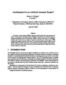
Figure 3. Environments #1 (top left), #2 (top right), #3 (bottom left) and #4 (bottom right) - shapes of the sequence of non-stationary fields in testing environments. For the six environments described above we did series of experiments by changing the parameters n (step 2 of the algorithm in Figure 1) – see Figure 4.
100%
80%
exogenic activation
60%
immune memory 40%
apoptosis
20%
0% 1
2
3
4
5
6
7
algorithm parameters settings
Figure 4. Division of population into activated individuals and individuals for apoptosis. Individuals that do not belong to any of the two subgroups are supposed to be an immune memory structure.
6
Every experiment of the seven from the Figure 4 was repeated through 50 epochs and in the later figures we always study average values of these 50 epochs. For the results estimation we used two measures proposed in [13]: Accuracy and Adaptability. Accuracy is a difference between the value of the current best individual in the population of the “just before the change” generation and the optimum value averaged over the entire run. Adaptability is a difference between the value of the current best individual of each generation and the optimum value averaged over the entire run. For both measures the smaller values are the better results.
avg value for 50 experiments .
4.1 Cyclic changes The results of cyclic changes are presented in Figure 5 (env. #1) Figure 6 (env. #2), Figure 6 (env. #3), and Figure 6 (env. #4) 600 500 400 300 200 100 0
1
2
3
4
5
6
7
A cc
204.77 69 197.45 81 193.94 93 148.48 26 116.58 97 186.32 81 308.59 04
A da
313.80 11 285.59 94 270.20 69 256.59 22 237.98 18 313.34 68 499.22 78 algorithm param eters settings
avg value for 50 experiments .
Figure 5. Results for experiments with 7 types of parameter settings performed with environment #1 (cyclic changes). 500 400 300 200 100 0
1
2
3
4
5
6
7
A c c 121.3524 103.236 86.55937 113.5491 158.3967 176.9148 307.5048 A da 178.1566 161.0866
151.08
171.7074 247.913 287.1489 451.4746
algorithm parameters s ettings
Figure 6. Results for experiments with 7 types of parameter settings performed with environment #2 (cyclic changes).
7
avg value for 50 experiments .
300 250 200 150 100 50 0
1
2
3
4
5
6
7
A c c 126.2156 91.96096 105.7489 120.4866 158.1875 155.6863 214.1541 A da 153.9885 109.2758 130.2685 148.6518 183.0292 192.706 254.9906 algorithm parameters s ettings
avg value for 50 experiments .
Figure 7. Results for experiments with 7 types of parameter settings performed with environment #3 (cyclic changes). 350 300 250 200 150 100 50 0
1
2
3
6
7
A cc
115.54
111.58
121.992
134.393 147.593
4
5
180.08
248.123
A da
132.629
127.841
139.452
153.853 173.617
206.509
286.283
algorithm parameters s ettings
Figure 8. Results for experiments with 7 types of parameter settings performed with environment #4 (cyclic changes). In the figures the best results, i.e. the smallest values of Accuracy and Adaptability are obtained for different algorithm parameters settings. However, every time they are better than for the algorithm where all individuals are activated or undergo apoptosis (settings No. 1) and better than the case where the number of activated individuals is small. For the environment #1 the best case is setting No. 5, the environment #2 – No. 3, the environments #3 and #4 – No. 2. 4.2 Non-cyclic changes The results of non-cyclic changes are presented in Figure 9 and Figure 10. In this case the best results are obtained for the settings where all individuals are activated or undergo apoptosis (setting No. 1) and the worst are in the case where the number of activated individuals is the smallest.
8
avg value for 50 experiments .
500 400 300 200 100 0
1
2
3
A cc
116.678
238.636
198.129
A da
318.358
318.691
313.618
4
5
6
7
231.441 246.568
267.038
255.539
370.477 342.734
360.645
450.882
algorithm parameters s ettings
avg value for 50 experiments .
Figure 9. Results for experiments with 7 types of parameter settings performed with environment #2 (non-cyclic changes). 350 300 250 200 150 100 50 0
1
2
3
6
7
A cc
147.973
154.305
150.403
177.849 167.947
4
5
182.84
272.352
A da
182.362
185.094
176.469
207.526 205.861
223.597
331.678
algorithm parameters s ettings
Figure 10. Results for experiments with 7 types of parameter settings performed with environment #4 (non-cyclic changes).
5. Conclusions Obtained results confirmed, that the individuals, which belong neither to activated group nor to the group for apoptosis play significant role in searching for optima in problems with cyclic changes only. Otherwise, when the problem changes in any non-cyclic way, the best approach is to divide the population simply into two groups: an activated individuals group and a group of individuals for apoptosis. For environments with cyclic changes we can not propose an effective general proportion between the groups in a population. Differences between the best settings of algorithm parameters indicate, that the best proportion depends of the type of changes in optimised environment and should be tuned individually.
9
But anyway, we can ascertain, that in case of cyclic changes a key to a success is a balance between explorative mechanisms of the algorithm (represented by phases of activation apoptosis) and – from the other side - a form of immune memory represented by the left group of individuals, that does not take part in both phases. Bibliography [1]
Nowell, A., Simon, H.A. Human Problem Solving. Prentice Hall, NJ 1972
[2]
Holland, J.H. Adaptation in Natural and Artificial Systems. MIT Press 1992
[3]
Gaspar, A., Collard, Ph. From Gas to artificial immune systems: Improving adaptation in time dependent optimization. Proc. of the 1999 Congress on Evolutionary Computation, 1859-1866
[4]
Wierzchoń, S.T. Multimodal optimization with artificial immune systems. M.A. Kłopotek, M.Michalewicz, S.T.Wierzchoń, eds, Intelligent Information Systems 2001. Physica-Verlag 2001, 167-179
[5]
Wierzchoń, S.T. Artificial immune systems in action: Optimization of nonstationary functions (in Polish). Proc. of the Workshop “Artificial Intelligence”, SzI’2001, Siedlce, Poland, December
[6]
Hofmeyr, S.A. An interpretative introduction to the immune system. Technical Report, Dept. of Computer Science, University of New Mexico, Albuquerque, NM, 1999
[7]
Wierzchoń, S.T. Artificial Immune Systems. Theory and Applications (in Polish). Warszawa 2001
[8]
Jerne, N.J. Towards a network theory of the immune system. Ann. Immunol. (Inst. Pasteur), 125C:373-389, 1974
[9]
de Castro, L.N., von Zuben, F.J. aiNet: An artificial immune network for data analysis. In: H.A. Abbas, R. A. Sarker, Ch. S. Newton (eds.) Data Mining: A Heuristic Approach. Idea Group Publishing, USA, 2001
[10] Perelson, A.S. Immune network theory. Immunological Review, 110: 5-36, 1989 [11] Bersini,H., Varela, F. The immune learning mechanisms: Reinforcement and recruitment and their applications. Computing with Biological Metaphors, Chapman Hall, 1994, 166-192 [12] Cobb, H.G., Grefenstette, J.J. Genetic algorithms for tracking changing environments. In: Proceedings of the Fifth International Conference on Genetic Algorithms. Morgan Kaufmann 1993 [13] Trojanowski,K., and Michalewicz, Z., Searching for optima in nonstationary environments, CEC’99, IEEE Publishing, pp.1843-1850
10