Searching for N2: How does Pressure Reduction Reduce Burst Frequency? D Pearson* M Fantozzi** Debora Soares*** T Waldron**** * David Pearson Consultancy Ltd, Cliff Road, Acton Bridge, Cheshire, CW8 3QY, UK,
[email protected] **Studio Fantozzi, Via Forcella 29, 25064 Gussago, Italy,
[email protected] ***Sabesp, 218, Dona Antonia de Queiroz, 01 307-010, Sao Paulo, Brazil,
[email protected] ****Wide Bay Water, 29 Ellengowan Street, Hervey Bay, Queensland, Australia,
[email protected]
Keywords:
Pressure Reduction; Burst Frequency; N2
Abstract Pressure management schemes are becoming increasingly popular - mainly because of the reduction of leakage in general and the reduction of background leakage in particular. But one of the biggest (economic) advantages of pressure reduction schemes is often overlooked: that is the significant reduction in burst frequency. Burst frequency data are normally only available to the utility and were only occasionally published. The authors have collected available data from utilities in Australia, Italy, the United Kingdom and Brazil for presentation in the paper. An analysis has been carried out to determine whether a general correlation exists between the reduction in pressure and the change in burst frequency. A new correlation factor, N2, has been introduced that will help practitioners to forecast the reduction in burst frequency when designing pressure reduction schemes. Based on these factors, the paper intends to stimulate further research in the economic impact of reduced burst frequency that is supposed to lead to a new understanding of the economic benefits of pressure reduction.
Introduction It is now generally accepted that pressure has a significant effect on leakage due to the reduction of flow rates from leaks. It is also accepted that reducing pressure will also reduce the level of background leakage, which is leakage from minor leaks generally below the level of detection. Most practicing engineers believe that burst frequencies are related to pressure but there have been limited studies into this relationship and because of this it is less well understood. This paper will provide a background to the understanding of the variation of burst frequencies and report on a number of case studies which have been investigated to establish the relationship between burst and pressure.
Relationship of flow rates to pressure The relationship between leakage and pressure has been the focus of many studies and several papers have been published on the topic. This work has established that flow rates are related to the power of the pressure. This power is referred to as N1, i.e. F = cPN1. This -1-
relationship follows on from the normal hydraulic relationship of flow from a fixed orifice where flow is proportional to the square root of the pressure – i.e. N1 = 0.5. Several studies have however shown that leakage from many distribution systems would imply a value of N1 greater than 0.5 and often greater than 1. Studies into this (May 1994; Lambert 2001) showed that this could be explained by the fact that some orifices are not of fixed dimensions and as the pressure grows the effective areas of these orifices increase. This phenomenon is known as the theory of Fixed and Variable Path Discharges (FAVAD). This work has suggested that N1 can be as high as 1.5 in the case of flexible joints involving gaskets and up to 2.5 in the case of leaks in some plastic pipe systems. The value of N1 will therefore vary with the level of leakage within a system and the proportion of rigid pipe within a system. This relationship has recently been further refined (Thornton and Lambert, 2005) and is reproduced in Figure1. P o w e r L a w E x p o n e n t N 1 v s IL I: p = % o f d e t e c t a b le r e a l lo s s e s o n r ig id p ip e s
P ower Law
Expon
1 .6
p=0%
1 .4 1 .2
p=20%
1 .0
p=40%
0 .8
p=60%
0 .6 0 .4
p=80%
0 .2
p=100%
0 .0 0
1
2
3
4
5
6
7
8
9
10
In f r a s t r u c t u r e L e a k a g e In d e x IL I
Figure 1 Predicting the N1 Exponent using ILI and % of detectable real losses on rigid pipes
Factors affecting burst frequencies Burst frequencies can vary significantly in various pipe materials and in different countries. Table 1 shows an analysis of burst frequencies that was produced from a survey carried out as part of a UK research programme (WaterUK 2000). Unfortunately, it has not been normal practice in such studies to relate burst frequencies to pressure. UK
Canada
West Germany
East Germany
Australia
Bulgaria
AC
11.5
7.3
6
34
8.4
141
Cast Iron
20.4
39.0
19
41
22.3
101
Ductile Iron
4.7
9.7
2
PE
3.1
PVC
9.4
Steel
12.5
1.6
10.3
74
6
14
9.0
21
74
9.8
1.2
93
Table 1 Burst frequencies of different pipe systems in different countries (no/100km/yr)
Burst frequencies in Eastern European countries appear to be significantly higher than Western Europe, Canada and Australia. Studies into burst frequencies show that there can be a number of causal factors, e.g.: •
Traffic loading/depth of installation -2-
-
•
Working pressure in relation to design pressure and surges
•
Age
•
Ground conditions and ground movement
•
Quality of installation
•
Quality of pipe materials.
•
Temperature and changes in temperature
Figure 2 shows a typical burst frequency versus age deterioration curve. This curve has been derived by establishing the burst frequency of pipe in a number of age bands. One difficulty that can arise with this analysis is that the pipe quality as supplied may vary. For example it is known that casting quality for pipe grade material deteriorated in the UK during the two major war periods. Also pipe performance may change due to the change in pipe material specifications – for example the quality of PVC pipe in the UK improved significantly when the fracture toughness requirement was built into the British Standard. Therefore pipe performance may not be homogeneous with time and discontinuities in performance with age may occur for a whole range of reasons. Number of failures for 1000m water main compared to age of pipes 9.0 8.5 8.0 7.5
Number of failures for 1000m water main
7.0 6.5 6.0 5.5 5.0 4.5 4.0 3.5 3.0 2.5 2.0 1.5 1.0 0.5 0.0 0
5
10
15
20
25
30
35
40
45
50
55
Age of pipes (year)
60
65
70
75
80
85
90
Failure
95
100
105
Trendline
Figure 2 Variation of pipe failure frequency with age for cast iron pipe (Bulgaria)
Similar factors to the ones described above will also affect service pipe performance. As a result of the factors discussed above the failure frequency of a distribution system at any one time will vary significantly in different parts of the network. Figure 3 shows a typical distribution of burst frequencies across a network. This shows (for example) that only 1% of the network fails at a frequency of 4 failures/km/year or more and 10% of the network fails at the frequency of 2 failures/km/year or more.
-3-
Burst Rate no/km/yr
10 9 8 7 6 5 4 3 2 1 0 0%
20%
40%
60%
80%
100%
Cum ulative % of netw ork
Figure 3 Typical distribution of mains failure frequencies across a distribution network
Relationship to pressure As discussed earlier practicing engineers will generally agree that when pressures are reduced on a system then the burst frequency reduces. Figure 4 shows a plot of pressure over a four month period at the beginning of 2001 on a district metered area (DMA) in the UK. The graph shows the diurnal variation due to demand on the system. A pressure control valve was installed and commissioned during the first week in February 2001 and pressures on the network were reduced by some 50m.
Figure 4 Pressure on district metered area in UK
Figure 5 shows the burst history for the same DMA . The columns are a histogram of the number of burst each month split between mains breaks, company service pipe bursts and customer supply pipe bursts. -4-
PRV commissioned
Figure 5 Burst history on district metered area
The graph clearly shows the dramatic reduction in burst frequency immediately following the commissioning of the pressure control valve in February 2001. Prior to the installation of the valve bursts were breaking out at a frequency of 3 per month. Following commissioning of the valve the burst frequency dropped to one every six months on average.
Figure 6 Pressure history at DMA showing pressure surge
-5-
Figure 6 shows the pressure history on a DMA and Figure 7 the corresponding burst history. There has been pressure reduction due to the installation of a pressure management valve in early 2002 but there was a pressure surge on one day in early May 2003. This single event caused 4 bursts - 2 mains bursts, a service pipe burst and customer supply pipe burst on a DMA which had only experienced 1 burst in the preceding 12 months. This reinforces the sensitivity of pipe failure to pressure fluctuations.
PRV commissioned Pressure surge
Figure 7 Burst history on DMA with pressure surge
The question is:– “can the burst frequency change be predicted and is it consistent?”. If a relationship between burst frequency and pressure can be established then it will be possible to develop economic models that look at the financial benefit of pressure control in terms of the reduction in the repair costs for an operating company. There have been only limited studies into this relationship. Studies carried out in the 1990s (Lambert 2001, Trow 2003) suggested that the change in burst frequency could be related to the change in pressure again to a power. This index has been referred to as N2. Thus:B1 / B0 = ( P1 / P0 ) N2 Where B1 = the burst frequency after pressure reduction B0 = the burst frequency before pressure reduction P1 = the pressure after pressure reduction P0 = the pressure before pressure reduction N2 = the power relationship Recent limited studies in the UK (UKWIR, 2003) on large grouped data sets concluded that “Long-term mains repair versus pressure do not show a convincing relationship between pressure and mains repair frequency”, but more detailed reading of this report reveals the recommendation that ‘ a square root relationship between burst frequency and pressure can be used as a pessimistic, worst case prediction for the effect of pressure management, -6-
knowing that the actual results are likely to be better, due to the stabilising effect of pressure management’. Thornton and Lambert (2005) suggest, from a number of limited studies, that N2 could be anywhere in the range 0.5 to 6.5. The ability to predict this relationship could have significant impact on the economic justification of pressure management schemes and the operating costs of water companies. The authors therefore considered it essential that further and more rigorous reviews are carried out. To this end the authors have started to collect data and carry out more detailed analyses to investigate the relationship and the factors that affect it.
Case Studies A number of utilities were approached as part of this study. Data was made available from:•
Bristol Water, UK
•
United Utilities, UK
•
SMAT, Italy
•
Umbra Acque, Italy
•
Sabesp, Brazil
•
Gold Coast Water, Australia
Qualitative review of the data reinforced the findings of the previous work and the results shown in Figures 4 - 7. Figure 8 shows the burst frequency for the area on the Gold Coast, Australia. This shows that the burst frequency reduced significantly when the pressure was reduced following the installation of a pressure control valve in September 2003. Burleigh DMA/PMA Main to Meter Corrective Maintenance 60
Service Breaks
Reduction in Service Breaks 75% Reduction in Mains Breaks 71%
Mains Breaks 50
No. Breaks
40
30
20
10
Month
Figure 8 Burst frequency history on DMA in Gold Coast, Australia
-7-
Mar-05
Dec-04
Sep-04
Jun-04
Mar-04
Dec-03
Sep-03
Jun-03
Mar-03
Dec-02
Sep-02
Jun-02
Mar-02
Dec-01
Sep-01
Jun-01
Mar-01
Dec-00
Sep-00
Jun-00
Mar-00
Dec-99
Sep-99
Jun-99
Mar-99
0
A protocol was developed for the data abstraction. Information on pressures and burst was abstracted from company information systems for a number of areas. Unfortunately one of the major difficulties in the study was having sufficiently long enough periods with stable pressure before and after pressure reduction to establish accurate burst frequencies. It had originally been suggested that three years of stable pressure would be needed to estimate accurate burst frequencies reliably. This was not possible with many of the locations that have been analysed in the project to date. In many cases the burst frequency post pressure reduction was such that no bursts actually occurred in the test period. This mitigates against the calculation of burst frequency. Data was abstracted from over 100 different locations. About 50 sites were found suitable after data cleansing. The results are summarised in the attached table.
Initial findings A number of relationships were hypothesised and tested. Firstly B1 / B0 = ( P1 / P0 ) N2 i.e.
N2 = ln ( B1 / B0) / ln ( P1 / P0 )
N2 values were calculated for over 50 sites. The values varied from 0.2 to 8.5 for mains breaks and from 0.2 to 12 for service pipe breaks. Figure 9 shows the distribution of N2 values The median and standard deviations are shown in Table 2.. 14 N2 mains
12
N2 services
N2
10 8 6 4 2 0 0
1
2
3 Po/P1
Figure 9 N2 values for different pressure changes
N2 (Median) SD
Mains 2.47 2.21
Services 2.36 3.29
Table 2 Median values of N2
-8-
4
5
Previous studies had implied that there may be a positive pressure at which the burst frequency would reduce to zero and the data analysed as part of this study supported this view. In order to investigate this, a revised relationship was hypothesised of the form:B1 / B0 = ( (P1 – P’) / (P0 – P’) ) N2 Where a is a positive pressure at which the burst frequency would be zero
Figure 10 shows the distribution of N2 with a 20m offset. It can be seen that there is a significant reduction in the range of N2 when an offset is used. Results are shown in Table 3 for two different values of P’. The results showed less variation as measured by the standard deviation and the range of the maximum and minimum values.
14 N2 mains
12
N2 services
N2
10 8 6 4 2 0 0
1
2
3
4
5
Po/P1
Figure 10 N2 values for different pressure changes using 20m offset
N2 (Median) SD Min Max
P’ = 10m Mains Services 1.94 1.71 1.57 2.33 0.16 0.16 5.89 8.66
P’ = 20m Mains Services 1.24 1.32 1.02 1.54 0.08 0.12 3.64 6.70
Table 3 Values of N2 with positive offset
The analysis appears to suggest that the offset could be of the order of 20m or more. However many systems (particularly in developing countries) have relatively high burst frequencies even though operating pressures are often below 20m.The use of an offset therefore needs further investigation. The graphs also indicate that N2 is smaller with larger changes of pressure. The variation of N2 could be due to a number of factors such as pipe material, installation and ground conditions. It may be feasible that this variation could be accounted for by a Fragility Index which could be related to these factors so that more accurate predictions of N2 could be made. The study of this will require more data.
-9-
Understanding the failure mechanism It is known that pipes fail due to a combination of a number of forces that act upon them when they are in service. Modes of failure for mains range from circumferential failure due to beam loading to longitudinal failure due to pressure. A multidimensional failure mode has been proposed (Rajani et al, 2000) which takes into account the different forces acting on a pipe. Figure 11 illustrates this in two dimensions where the Y axis is the traffic loading and the X the internal pressure. The Z axis represents the probability of failure. If pressure was greater than Pmax then the pipe would fail under the pressure failure mode. If the traffic loading was greater than Tmax then the pipe would fail under beam bending. There will be a envelope joining point Pmax and Tmax where the pipe will fail from either or a combination of these two failure modes. When the pipe is subjected to a combination of pressure and traffic loading which is outside the envelope the pipe will fail. When the combination is within the envelope the pipe will continue to perform. The shape of the envelope will be a function of pipe material, corrosion, graphitisation and tuberculation as well as design and installation parameters. As the pipe ages and, say, the wall thins due to corrosion, the value of Pmax and Tmax (i.e. the loadings at the point of failure) will reduce and hence the failure envelope will “move” towards the origin. A pipe will have a duty point at the average pressure and traffic loading at the site (say at point A). In practice the point at which the pipe operates will be fuzzy (represented by the two dimensional normal probability density function (pdf) “bell” shape on the figure) due to the stochastic nature of pressure and traffic loading. The shape of the pdf will be a function of the variation in pressure and traffic loading. A pressurised network which subjects the pipe to surges will have a greater range and, hence, a wider probability density function compared to a gravity system. When a pipe is initially installed this “duty” point will be some way within the envelope The distance between Point A and the envelope will be related to the safety factor built into the design of the pipe and the choice of pressure rating. This point will be at such a distance from the envelope that the probability of failure is very low.
Failure Envelope Duty point B (45m, 40t) T max (80t) Duty point A (75m, 40t)
0
Failure
100 90
20
80 70
40 60 Pressure
60
50 40
80
30 20
100
Pmax (100m)
Traffic Loading
10
120
0
Figure 11 3D plot of failure envelope and duty points for pressure pipe
- 10 -
Reducing the average pressure experienced by the pipe will move it to duty Point B. As can be seen this moves the pipe further into safety away from the failure envelope and hence reduces the burst frequency. If the change in pressure was sufficient to move the pdf of Point B sufficiently away from the failure envelope then the burst frequency would be reduced to zero for a period until the pipe properties deteriorated such that the failure envelope moved to overlap with the pdf of Point B. This hypothesis would support the use of an offset to the pressure-burst relationship. As the distance between and duty point and the failure envelope reduces with age, the burst frequency will increase as the pipe experiences combinations of pressure and traffic loading that push it over the failure envelope. This effect has been modelled as part of an EU sponsored research programme (Hadzilacos et al, 2000). Analysis developed as part of this project showed (Camarinopoulos et al, 1999) how this results in the failure probability increasing in the form of an S Curve (Figure 12). This will manifest itself in an increase in the burst frequency with time as shown in Figure 2. By moving the duty point away from the failure envelope the performance of the pipe will be restored – equivalent to moving to a much younger pipe (see Figure 2). The economic life of the pipe will therefore be extended perhaps by a matter of tens of years.
100% Failure probability
Time (years) Figure 12 “S” Curve of failure probability with time
Modes of failure for some service connections, e.g. ferrule blow out, will be different and there has been little research into the mechanism of these failures. Since the shape of the curve is a function of pipe materials and site conditions then the effect of pressure reduction will differ in different situations.
Economic benefit of burst reduction In the UK, the benefit of pressure management schemes is currently evaluated based on the savings that would accrue in leakage from the reduction in background losses and burst flow rates. Companies will install pressure management until the cost of the installation is greater than the benefit that accrues from these leakage savings either in the cost of water or the deferment of new schemes. Figure 13 shows a typical curve of the diminishing return as pressure management schemes are deployed within a company. A point will be reached when it is not worth installing any further pressure management schemes. This paper has shown however that burst frequency will also reduce when pressure management is deployed. This will bring additional savings from reductions in customer contact, inspections, repairs, leakage detection costs and increased life of the asset. Studies carried out by the authors using economic leakage models have shown that when these additional cost benefits are brought into the equation then it is economic to carry out pressure management to a significantly lower level than previously assessed. - 11 -
AZNP(m) 50.0 49.0 48.0 47.0 46.0 45.0 44.0 43.0 42.0 41.0 40.0 1
5
9
13
17
21
25
29
33
37
41
45
49
53
57
61
65
69
73
77
81
85
89
93
97 101 105 109 113 117 121 125 129
Scheme
Figure 13 Reduction in average pressure with installation of pressure control valves
Conclusion The paper has presented data from studies of burst frequencies following pressure reduction. These studies have clearly demonstrated that burst frequencies reduce following pressure reduction. The data has been abstracted and a number of hypothesised relationships tested. In the case of a simple index relationship the median value of the index N2 was 2.47 and 2.36 for mains and service pipe breaks respectively. When an offset at which the burst frequency would be reduced to zero was introduced then the variation of N2 reduced. The median value of N2 when the offset was 20m was 1.24 and 1.32 for mains and service pipe breaks respectively. Further work is recommended into:•
The impact of pressure fluctuations
•
The effect pf pressure range as well as maximum pressures
•
Understanding burst frequencies in low pressure networks
•
Factors (such as mains material, age etc) that may explain the variability in the N2 values
A model of pipe failure has been proposed that may provide a framework for understanding the variation in burst failure in relation to pipe material and design. There are significant benefits from the savings that could accrue from burst reductions and it is suggested that this is an area that warrants continued investigation. The authors are willing to continue this work and would encourage the submission of further data to assist in the development of the understanding into the relationship between pressure and burst frequency. To this end the authors have developed a protocol for the collection of data. A standard piece of free software (N2Calc) is also available for the submission of data.
- 12 -
Acknowledgments The authors would like to thank the companies who have been willing to make data available for the studies described in this paper. In particular United Utilities and Bristol Water in the UK, Sabesp in Brazil, Gold Coast Water in Australia and SMAT and Umbra Acque in Italy. The work could not have been carried out without access to this data. The authors would also like to thank the members of the Pressure Management Team of the IWA Water Loss Task Force, and in particular R. Liemberger, for their encouragement in carrying out these studies.
References Camarinopoulos, L.., Chatzoulis, A., Frondistou-Yannas, S. and Kallidromitis, V. (1999) Assessment of the timedependent structural reliability of buried water mains. Reliability Engineering and System Safety 65 (1999) 41-53 Elsevier Science Farley, M. and Trow, S. (2003) Losses in water distribution networks. IWA, 2003, ISBN 1 900222 11 6 Hadzilacos, T., Kalles, D., Preston, N., Melbourne, P., Camarinopolous, L., Eimermacher, M., Kallidromitis, V., Frondistou-Yannas, S. and Saegrov, S. (2000) Utilnets: a water mains rehabilitation decision support system. Computers, Environment and Urban Systems 24 (2000) 215-232 Elsevier Science Lambert, A. (2001) What do we know about pressure:leakage relationships. IWA Conference, BRNO, 2001 ISBN 80-7204-197-51 Lambert, A. and Thornton, J. (2005) Progress in practical prediction of pressure:leakage, pressure:burst frequency and pressure:consumption relationships. IWA Leakage2005 Conference, Halifax (Canada) May, J. (1994) Pressure dependent leakage. World Water and Water Engineering, October 1994 Rajani, B. and Makar, J, (2000) A methodology to estimate remaining service life of grey cast iron water mains. Can Journal of Civil Eng 27 p1259-1272 UKWIR (2003) Leakage index curve and the longer term effects of pressure management. Report 03/WM/08/29, 2003, ISBN 1084057-280-9 WaterUK (2000) Plastic Pipe Group Research Programme Workshop, York
- 13 -