Atmosphere 2014, 5, 399-419; doi:10.3390/atmos5020399 OPEN ACCESS
atmosphere ISSN 2073-4433 www.mdpi.com/journal/atmosphere Article
Seasonal and Diurnal Variations of Total Gaseous Mercury in Urban Houston, TX, USA Xin Lan 1,*, Robert Talbot 1, Patrick Laine 2, Barry Lefer 1, James Flynn 1 and Azucena Torres 1 1
2
Institute for Climate and Atmospheric Sciences, Department of Earth & Atmospheric Sciences, University of Houston, Houston, TX 77204, USA; E-Mails:
[email protected] (R.T.);
[email protected] (B.L.);
[email protected] (J.F.);
[email protected] (A.T.) Portnoy Environmental Incorporation, Houston, TX 77043, USA; E-Mail:
[email protected] (P.L.)
* Author to whom correspondence should be addressed; E-Mail:
[email protected] (X.L.); Tel.: +1-347-276-3889. Received: 10 March 2014; in revised form: 22 April 2014 / Accepted: 28 April 2014 / Published: 30 May 2014
Abstract: Total gaseous mercury (THg) observations in urban Houston, over the period from August 2011 to October 2012, were analyzed for their seasonal and diurnal characteristics. Our continuous measurements found that the median level of THg was 172 parts per quadrillion by volume (ppqv), consistent with the current global background level. The seasonal variation showed that the highest median THg mixing ratios occurred in summer and the lowest ones in winter. This seasonal pattern was closely related to the frequency of THg episodes, energy production/consumption and precipitation in the area. The diurnal variations of THg exhibited a pattern where THg accumulated overnight and reached its maximum level right before sunrise, followed by a rapid decrease after sunrise. This pattern was clearly influenced by planetary boundary layer (PBL) height and horizontal winds, including the complex sea breeze system in the Houston area. A predominant feature of THg in the Houston area was the frequent occurrence of large THg spikes. Highly concentrated pollution plumes revealed that mixing ratios of THg were related to not only the combustion tracers CO, CO2, and NO, but also CH4 which is presumably released from oil and natural gas operations, landfills and waste treatment. Many THg episodes occurred simultaneously with peaks in CO, CO2, CH4, NOx, and/or SO2, suggesting possible contributions from similar sources with multi-source types. Our measurements revealed that the mixing ratios and variability of THg were primarily controlled by nearby mercury sources.
Atmosphere 2014, 5
400
Keywords: mercury; total gaseous mercury; urban air quality; emission inventories
1. Introduction Mercury is a toxic environmental pollutant [1]. It is mobilized from deep reservoirs in the Earth to the atmosphere, where it then deposits to terrestrial systems and water bodies. Mercury in the water can be transformed into methylmercury, a much more toxic form that accumulates in fish and shellfish [2]. Humans are exposed to mercury poisoning mainly by consuming contaminated seafood. In these processes, the atmosphere serves as a major pathway for mercury transport from sources to receptors. Thus, it is important to quantify and characterized mercury in the atmosphere. In the atmosphere, mercury exists in three chemical forms: gaseous elemental mercury (GEM = Hg°), gaseous oxidized mercury (GOM), and particulate bound mercury (PBM). Gaseous elemental mercury is the most abundant chemical from, which accounts for about 95% of total atmospheric mercury [3–5]. Atmospheric mercury is emitted from both natural and anthropogenic sources. Natural sources include volcanoes and geothermal areas, mercury enriched soils, wild fires, and the ocean [6–12]. Major anthropogenic sources include coal combustion, industrial and commercial boilers, electric arc furnaces, cement production, and waste treatment facilities [13]. The National Emission Inventory (NEI) from the U.S. Environmental Protection Agency (EPA) reports that 59 tons out of 61 tons of total mercury emissions in the U.S. are from stationary sources. Combustion of fossil fuels is considered as the major anthropogenic source of atmospheric mercury; coal-fired utility boilers alone account for 49% of anthropogenic emissions [13]. The sources of atmospheric mercury are just beginning to be characterized and quantified; large uncertainties remain in various mercury sources, such as on-road vehicles, oil refineries, and other industrial facilities [14–17]. Ambient mercury levels have been assessed through careful measurements. A 10-year (1995–2005) measurement at 11 sites from the Canadian Atmospheric Mercury Measurement Network (CAMNet) reported that the averaged THg (THg = GEM + GOM) concentration was 1.58 ng·m−3 (177 ppqv) [18]. Long-term measurements have also been conducted at two European background sites [19]. The 6-year (1998–2004) mean of THg concentration at these coastal sites were of 1.72 ng·m−3 (193 ppqv) and 1.66 ng·m−3 (186 ppqv) at Mace Head, Ireland and Zingst, Germany, respectively. In a recent review, Sprovieri et al. [20] concluded that the current background concentration of atmospheric mercury was 1.5–1.7 ng·m−3 (168–190 ppqv) in the Northern Hemisphere. The temporal and spatial variations of atmospheric mercury are of critical importance as it can help to understand the physical transformations of mercury species or chemical sources and sinks. A study of CAMNet data showed a common diurnal pattern for most rural sites with minimum concentrations right before sunrise and maximum concentrations around solar noon, which was attributed to nighttime depletion in the lowermost atmosphere [21]. A recent report on the U.S. Atmospheric Mercury Network (AMNet) found similar pattern [22]. GEM dissolution into dew at night and re-volatilization in the early morning were considered to be dominant factors controlling this diurnal pattern, which was similar to the results for New Hampshire reported by Mao and Talbot [23,24].
Atmosphere 2014, 5
401
In urban areas, however, the mixing ratios of atmospheric mercury, and its seasonal and diurnal variation patterns are very different from rural sites, due to complex anthropogenic emissions, topography and meteorology. The averaged GEM concentration in urban Detroit was reported to be 2.5 ng·m−3 (280 ppqv) for 2004 [25]. The seasonal variation pattern showed the highest seasonal GEM concentration in summer and the lowest concentration in winter, which was different from most rural site measurements [21,22]. A study in urban Birmingham, Alabama, reported averaged GEM concentration of 2.12 ng·m−3 (237 ppqv) for the 2005–2008 period [26]. Measurements in Salt Lake City showed that the median GEM concentration was 226 ppqv for the 2009–2010 period [22], which was also higher than many rural site measurements. In general, four different diurnal patterns are frequently reported in the literature, concerning the relative importance of surface emission rate versus the deposition rate: (1) Mercury steadily decreases at night and reaches its minimum level just before sunrise, then gradually increases to reach a maximum level at noon or in the early afternoon. The decrease at night may be related to dry deposition or uptake by wet surfaces. This pattern was observed frequently at rural and remote areas, such as some of the CAMNET and AMNet sites. (2) Mercury accumulates overnight under the influence of a low nocturnal boundary layer, and reaches its maximum before sunrise, followed by a rapid decrease after sunrise and a daily minimum in the afternoon. This pattern most commonly occurs in urban sites where strong local and regional emissions are predominant [27–29]. (3) Mercury rapidly increases right after sunrise, followed by a gradual decrease in the later hours. The rapid increase after sunrise was due to the erosion of the residual layer with elevated mercury concentrations brought down to the surface. This pattern likely occurs in rural or suburban areas, and some urban areas with special topographies [26,30–32]. (4) Mercury exhibits very small diurnal variation at elevated sites above the nocturnal boundary layer [33], and in the marine environment [23,34]. This study characterized the seasonal and diurnal variations of total gaseous mercury (THg = GEM + GOM) in the Houston area, and investigated the factors governing those changes. Understanding mercury pollution in the Houston area is complex and unique because of its distinct industrial emissions and changing meteorological conditions. Approximately 400 refineries surround the Galveston Bay in Houston, and a multitude of other industrial facilities are distributed across the region. Numerous mercury sources were reported in the 2008 EPA NEI [35] in this area (Figure 1). The Formosa Plastics Company, located to the southwest of Houston, was reported to have 1.068 metric tons of mercury emissions per year. The W.A. Parish plant, one of the largest coal-fired electrical generating plants in the U.S., is located southwest of Houston and emits 265 kg/yr. Several mercury sources, such as oil refineries and waste treatment facilities, are congregated in the Houston Ship Channel area, the vicinity to the northeast and east of our monitoring site. To the southeast of Houston, Texas City also has industrial facilities that are reported as mercury sources. The Houston-The Woodlands-Sugar Land is the fifth-largest metropolitan area in the U.S. with over 6 million people [36]. There is a dense highway/roadway network with heavy traffic in the metropolitan area. In addition to these large number of potential mercury sources, the meteorological conditions, especially the bay and sea breezes complicate the regional and local transport of mercury. Atmospheric mercury was observed in the Houston area for the first time during the Texas Air Quality Study II (TexAQS II, 2005–2006). Measurements on the Moody Tower (MT) observing site on the University of Houston campus captured extremely high concentrations of PBM (79 pg·m−3)
Atmosphere 2014, 5
402
downwind of the Galveston Bay refinery complex [37]. During TexAQS II concentrated plumes of GEM (up to 28,000 ppqv or 250 ng·m−3) were observed repeatedly in the Houston Ship Channel area and once in the Beaumont-Port Arthur area [38]. However, no continuous measurements were reported from this metropolitan area to quantify the average ambient levels and temporal variations. In fact, few long-term ambient mercury measurements are available for urban environments. Our group has been conducting measurements of atmospheric mercury in the Houston area since August 2011. This study is our first report based on 14 months of continuous measurements. Our aim is to provide important information on mercury pollution in a heavily polluted urban area to help evaluate the regional mercury budget, and further facilitate regional modeling and policy-making processes. Figure 1. Facility emission sources around MT site from 2008 NEI facility data. A satellite image of the red box area is provided in the supporting material (Figure S1) for details of Houston Ship Channel area. 31.5
31.0
Latitude, North
30.5
30.0
Houston ship channel MT
Trinity Bay
29.5
Texas City 29.0
28.5 -97.0
-96.5
-96.0
-95.5 Longitude, East
-95.0
MT Road Water Line 0.001-1 kg/yr 1-10 kg/yr 10-100 kg/yr 100-200 kg/yr 200-300 kg/yr >300 kg/yr -94.5
-94.0
2. Results and Discussion 2.1. Seasonal and Diurnal Variations The complete time series of THg is presented in Figure 2. The median level of THg in Houston was 172 ppqv (181 ± 63 ppqv for mean ± S.D.) during our observation period (see Figure S2 and Table S1 for more statistical details), which was in agreement with the current background level in the Northern Hemisphere [20], but slightly lower than other urban sites with mercury levels higher than 2 ng·m−3 (224 ppqv) [22,25,28,39,40]. The majority of THg observations fell within the range of 148 ppqv (10th percentile) to 215 ppqv (90th percentile). The maximum THg mixing ratio, however, was as high as
Atmosphere 2014, 5
403
4876 ppqv, exceeding 25 times the current global background level. The minimum level was 80 ppqv, which occurred with southerly wind that brought cleaner air from the Gulf of Mexico into urban Houston. A prominent feature of THg in the Houston area was the frequent occurrence of large THg spikes (Figure 2b). From 14-month measurements, we documented 81 well-developed spikes with THg levels higher than 300 ppqv, 34 of which were higher than 500 ppqv. Extremely large peaks with THg levels higher than 1000 ppqv were observed 12 times, and six of them were higher than 3000 ppqv. The time scale of elevated mercury in these spikes ranged from 30 minutes to a few hours. As a consequence of the THg spikes, the standard deviations of our data reached 63 ppqv, which was comparable with other urban sites measurements, such as Salt Lake City (95 ppqv [22]) and Reno (45–90 ppqv [39]). Figure 2. Complete time series of THg from MT measurements. (a) and (b) show the same data with different ranges in y axis. 700
a
THg (ppqv)
600 500 400 300 200
THg (ppqv)
100 4500 4000 3500 3000 2500 2000 1500 1000 500 9/1/11
b
11/1/11
1/1/12
3/1/12
5/1/12
7/1/12
9/1/12
Seasonal median levels of THg were 178 ppqv (179 ± 54 ppqv for mean ± S.D.), 161 ppqv (161 ± 80 ppqv), 172 ppqv (172 ± 26 ppqv), and 185 ppqv (186 ± 32 ppqv) for fall 2011, winter 2011, spring 2012 and summer 2012, respectively. The monthly median THg values are displayed in Figure 3. Unlike many other ambient mercury measurements, which show higher mercury in winter time [21,22], high THg in Houston area occurred in the warm seasons (June to October). It is obvious that the frequent occurrences of large THg spikes during the warm seasons, especially in August, September and October, contributed to the elevated THg levels. The great enrichments in episodic THg spikes suggested that the large pollutant plumes originated from the nearby industrial/urban emission sources. Mercury emissions from anthropogenic sources are closely linked to energy production, especially from coal-fired power plants, the largest anthropogenic mercury source in U.S. [13]. Enhanced energy production is expected in the Houston area in summer and fall. The high ambient air temperature requires energy to operate air-conditioning units. As a consequence, the ambient THg levels may increase. To illustrate this point, the state-level energy data achieved from Energy Information
Atmosphere 2014, 5
404
Administration (EIA) is presented in Figure 3. The monthly total energy produced in warm months was 50%–100% higher than in the cold months (The correlation coefficient between monthly median THg and monthly median energy production is 0.735, which is statistically significant (p ≤ 0.005)). Besides the fluctuations in mercury sources, we noticed some changes in potential sinks. Mercury deposition in rain water has been commonly reported [41–43], indicating rainfall as an important removal mechanism for atmospheric mercury. The precipitation in Houston was observed to be consistently higher in the period from December 2011 to March 2012 (Figure 3), which coincided with low wintertime THg.
THg (ppqv)
260 240 220 200 180 160 140 8/11
10/11
12/11
2/12
4/12
6/12
8/12
7 10/12 ×10
500 400 300 200 100
Precipitation (mm)
2.8 2.6 2.4 2.2 2.0 1.8 1.6 1.4 1.2
280
Generator Production (Megawatt Hour)
Figure 3. Monthly medians of THg, energy production and precipitation.
0
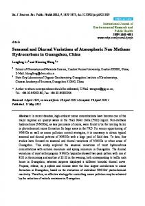
Precipitous day-to-day peaks and valleys variations were also observed as another outstanding feature of THg signal. Hourly median THg mixing ratios are displayed in Figure 4a. Despite the differences in variation amplitudes, diurnal variation patterns in fall, winter and spring were generally similar. Their diurnal patterns show a period with increasing THg levels starting around 16:00–18:00 local standard time (LST) and lasting for 2–4 hours, followed by a period with relatively constant THg levels. A sharp enhancement of THg levels started at around 04:00 LST, and then the THg reached a daily maximum at 07:00–09:00 LST. The summer diurnal pattern, however, appeared to be very different from other seasons. The THg level in summer gradually increased throughout the whole night and reached its maximum at about 07:00 LST, indicating an accumulation process of THg. Summertime had the highest THg mixing ratios during a day, and the largest diurnal variation amplitude (about 30 ppqv) among the four seasons. To conclude, the THg levels were higher at night than during the daytime. The maximum levels appeared right before sunrise, followed by rapid decreases after sunrise, and daily minimum shortly after noon. Similar diurnal patterns were observed in other urban cities, such as Guiyang, China [27], Detroit, U.S. [28], and Toronto, Canada [29]. It is interesting to note that the THg mixing ratio reached its diurnal maximum at about 07:00 LST in fall, spring and summer, while it was two hours later in winter. This phenomenon was related to the diurnal development of the PBL (Figure 4b). The PBL heights started increasing at about 06:00–07:00 LST for spring and summer and two hours later for winter. The rapid enhancements of PBL height in early morning can facilitate air mixing in three-dimensions and dilute the ambient THg within the boundary layer, and thus caused striking decreases of THg at the same time. The rate of decrease in
Atmosphere 2014, 5
405
summer was the largest (7.0 ppqv·h−1), compared to those in winter (1.9 ppqv·h−1), spring (2.6 ppqv·h−1), and fall (4.6 ppqv·h−1). The high PBL height in daytime then contributed to the low THg mixing ratios, especially in the afternoon. This phenomenon suggested that the residual layer was not a significant source for THg in Houston; instead, the industrial/urban emissions from the surface were more prominent. Figure 4. Seasonally diurnal variations of THg (a), PBL height (b) and horizontal wind speed (c). Data shows the median values with 5 min. time interval. The top x axis shows time in LST and the bottom x axis shows time in UTC. LST = UTC − 6:00. LST 18:00 200
22:00
2:00
6:00
a
14:00
18:00
Fall 2011 Winter 2011 Spring 2012 Summer 2012
190 THg (ppqv)
10:00
180 170 160 1800 1600
Winter UTC 2011 Spring 2012 Summer 2012
b
PBL (m)
1400 1200 1000 800 600 400 200
Wind Speed (m/s)
6.0
c
Fall 2011 Winter 2011 UTC Spring 2012 Summer 2012
5.5 5.0 4.5 4.0 3.5 3.0 2.5 00:00
04:00
08:00
12:00 UTC
16:00
20:00
00:00
Atmosphere 2014, 5
406
However, some features of the diurnal THg variations cannot only be explained by the PBL height propagations, for example, the summertime THg mixing ratios were the highest during all times of the day even though the daytime PBL heights were the highest. It was observed that the diurnal variations of horizontal wind speeds were anti-correlated with THg levels most of the time (Figure 4c, median wind speeds were calculated using scalar values). High horizontal wind speeds can enhance horizontal mixing of polluted air with cleaner ambient air, and effectively advect the pollutants away from the urban area. The summertime wind speed was the lowest of all seasons, and the especially low wind speeds at night supported the accumulation of THg and caused high summertime THg mixing ratios. In spring, low wind speeds were observed at 04:00–07:00 LST, which probably contributed to the high THg mixing ratios in this period. The energy production/consumption, precipitation, PBL height, and horizontal wind speed played important roles in the seasonal and diurnal variations of THg; however, we cannot quantify the contribution of each factor from our observations. Regional modeling with a good emission inventory and dynamic processing is necessary for further investigation. It is unclear whether photochemical reactions play an important role in determining THg mixing ratios in the Houston area. Previous research suggests that the main sink of GEM in the atmosphere is oxidation to GOM [44]. The GOM then can attach to particles and be transformed to PBM. Both GOM and PBM are easily removed from the air via wet and dry deposition [21,45], which will eventually reduce the mixing ratio of THg. From our observations, the diurnal THg mixing ratios remained constant from 12:00 LST to 16:00 LST in fall, spring and summer. During these times, photochemical reactions should be actively changing due to the fluctuations of solar radiation and variations in the abundance of oxidants. The effect of photochemical reactions may be obscured due to complex local emissions and meteorological conditions. Natural sources can also influence the seasonal and diurnal variations of ambient THg levels; however, we are unable to quantify the contributions of natural emissions in metropolitan Houston due to a lack of direct measurements. However, a large portion of vegetation in the Houston area is evergreen; with no snow in winter, we expect small contributions from natural emissions to the THg seasonal variations. 2.2. Wind Induced Influences In addition to the wind speed, the wind direction also exerts considerable impacts on THg variations, suggesting the importance of local/regional transport. In Figure 5, the percentage values on the R axis shows the frequency (%) of THg coming from a certain range (22.5°) of wind directions. The predominant wind directions in our observed period were south and southeast directions (120°–190°) (Figure 5a), which were from the Gulf of Mexico. The overall frequency from these directions accounts for about 40%, after summing up the percentage values from 120°–190° directions in Figure 5a. Cleaner air masses with especially low THg levels (4 m/s, occurred in December) yielded THg levels ≥ 150 ppqv, and CO levels ≥ 125 ppbv. In comparison, consistent southerly winds with high wind speeds (occurred in April) produced THg levels as low as 120 ppqv and CO levels as low as 85 ppbv. The large discrepancies between southerly air and northerly air highlight the significance of local urban/industrial influences on elevated THg mixing ratios in the Houston area. The sea breeze exerted significant and complex impacts on THg levels in the Houston area. The sea breeze is driven by diurnally uneven heating in coastal areas, which produces warmer temperatures over land than over water during the day, and cooler land temperatures at night [46]. As a result, a sea breeze is produced when the air flows from the sea to the land at low altitude (