Second Order Sufficient Optimality Conditions for a Control Problem ...

Second Order Sufficient Optimality Conditions for a Control Problem with Continuous and Bang-Bang Control Components: Riccati Approach Nikolai P. Osmolovskii

1

Systems Research Institute, Polish Academy of Sciences ul. Newelska 6, 01-447 Warszawa, Poland and University of Podlasie, Institute of Mathematics and Physics, ul. 3 Maja 54, 08-110 Siedlce, Poland and Polytechnika Radomska and Akademia Podlaska, Poland [email protected] Helmut Maurer

2

Westf¨alische Wilhelms–Universit¨at M¨ unster, Institut f¨ ur Numerische und Angewandte Mathematik, Einsteinstr. 62, D–48149 M¨ unster, Germany, [email protected] Abstract Second order sufficient optimality conditions for bang-bang control problems in a very general form have been obtained in [15, 21, 13, 12, 1]. These conditions require the positive definiteness (coercivity) of an associated quadratic form on the finite-dimensional critical cone. In the present paper, we investigate similar conditions for optimal control problems with a control variable having two components: a continuous unconstrained control appearing nonlinearly and a bang-bang control appearing linearly and belonging to a convex polyhedron. The coercivity of the quadratic form can be verified by checking solvability of an associated matrix Riccati equation. The results are applied to an economic control problem in optimal production and maintenance, where existing sufficient conditions fail to hold. Key Words: bang–bang control, Pontryagin minimum principle, second order sufficient conditions, critical cone, quadratic form, strengthened Legendre condition, Riccati equation, economic control problem

1

Introduction

The classical sufficient second order optimality conditions for an optimization problem with constraints require that the second variation of the Lagrangian 1 2

This work was partially supported by the grant RFBR 04-01-00482 Supported by the Deutsche Forschungsgemeinschaaft under grant MA 691/18-1

1

be positive definite on the cone of critical directions. In this paper, we investigate sufficient quadratic optimality conditions of such type for optimal control problems with a vector control variable having two components: a continuous unconstrained control appearing nonlinearly in the control system and a bang–bang control appearing linearly and belonging to a convex polyhedron. In the pure bang-bang case, where all control components appear linearly, second order necessary and sufficient optimality conditions in a very general form have been obtained in Milyutin, Osmolovskii[15], Osmolovskii [21], Agrachev, Stefani, Zezza [1], and Maurer, Osmolovskii [13, 12, 24]. Two alternative approaches were developed to establish sufficiency: (1) check the positive definiteness of an associated quadratic form on the finite-dimensional critical cone; (2) verify second-order sufficieent conditions for an induced finitedimensional optimization problem with respect to switching times and free final time. Second order sufficient optimality conditions for control problems where the control variable appears nonlinearly, more precisely, where the strict Legendre condition holds, have been given, e.g., in Malanowski [8], Maurer [9], Maurer, Pickenhain [14], Milyutin, Osmolovskii [15], and Zeidan [28]. Here, one way to check the positive definiteness of the quadratic form is by means of the solvability of an associated Riccati equation. In this paper, we investigate a class of control problems having two control components, a continuous and a bang–bang component. Such control problems are frequently encountered in practice. Our aim is to obtain second-order sufficient optimality conditions for this class of control problems. It does not come as a surprise that the proof techniques for obtaining sufficient conditions combine the above mentioned methods in the pure bang–bang case and the case where the strict Legendre condition holds. For simplicity, we shall consider control problems on a fixed time interval. In Section 2, we give a statement of the control problem with continuous and bang-bang control components (main problem), formulate the minimum principle (first order necessary optimality condition) and introduce the notion of bounded-strong local minimum. In Section 3, we present second-order sufficient optimality conditions (SSC) for a bounded-strong minimum in the problem. The main result in Theorem 3.3 is stated without proof, which is very similar to the proof in the bang-bang case; cf. Milyutin, Osmolovskii [15] and Osmolovskii, Maurer [24], Part 1. In Section 4, we give criteria for the positive definiteness of the quadratic form on the critical cone in terms of solutions to a matrix Riccati equation which may be discontinuous at the switching times. In Section 5, the main result in Theorem 4.1 is applied to an economic control problem for optimal production and maintenance which was introduced by Cho, Abad and Parlar [4]. We will show that the numerical solution obtained in Maurer, Kim, and Vossen [10] satisfies the second order test derived in Section 4 while existing sufficiency results fail to hold.

2

2

Control problem on a fixed time interval

2.1

The main problem

Let x(t) ∈ IRd(x) denote the state variable and u(t) ∈ IRd(u) , v(t) ∈ IRd(v) the control variables in the time interval t ∈ [t0 , tf ] with fixed initial time t0 and final time tf . We shall refer to the following optimal control problem (1)–(4) as the main problem: Minimize

J (x(·), u(·), v(·)) = J(x(t0 ), x(tf ))

(1)

subject to the constraints x(t) ˙ = f (t, x(t), u(t), v(t)), u(t) ∈ U, (t, x(t), v(t)) ∈ Q, F (x(t0 ), x(tf )) ≤ 0, K(x(t0 ), x(tf )) = 0, (x(t0 ), x(tf )) ∈ P,

(2) (3)

where the control variable u appears linearly in the system dynamics, f (t, x, u, v) = a(t, x, v) + B(t, x, v)u .

(4)

Here, F, K, a are column-vector functions, B is a d(x) × d(u) matrix function, P ⊂ IR2d(x) , Q ⊂ IR1+d(x)+d(v) are open sets and U ⊂ IRd(u) is a convex polyhedron. The functions J, F, K are assumed to be twice continuously differentiable on P and the functions a, B are twice continuously differentiable on Q. The dimensions of F, K are denoted by d(F ), d(K). By ∆ = [t0 , tf ] we shall denote the interval of control and use the abbreviations x0 = x(t0 ),

xf = x(tf ),

p = (x0 , xf ).

A process Π = {(x(t), u(t), v(t)) | t ∈ [t0 , tf ] } is said to be admissible, if x(·) is absolutely continuous, u(·), v(·) are measurable and bounded on ∆ and the triple of functions (x(t), u(t), v(t)) together with the endpoints p = (x(t0 ), x(tf )) satisfies the constraints (2) and (3). Definition 2.1 An admissible process Π affords a Pontryagin local minimum, ˜ ≥ J (Π) for if for each compact set C ∈ Q there exits ε > 0 such that J (Π) ˜ = {(˜ all admissible processes Π x(t), u˜(t), v˜(t)) | t ∈ [t0 , t1 ] } such that (a) max |˜ x(t) − x(t)| < ε; ∆

(b)

R

∆

|˜ u(t) − u(t)| dt < ε;

R

|˜ v(t) − v(t)| dt < ε;

∆

(c) (t, x˜(t), v˜(t)) ∈ C a.e. on ∆. 3

2.2

First order necessary optimality conditions

Let Π = {(x(t), u(t), v(t) | t ∈ [t0 , tf ] } be a fixed admissible process such that the control u(t) is a piecewise constant function and the control v(t) is a continuous function on the interval ∆ = [t0 , tf ]. In order to make the notations simpler, we do not use such symbols and indices as zero, hat or asterisk to distinguish this trajectory from others. Denote by θ = {t1 , . . . , ts }, t0 < t1 < . . . < ts < tf , the finite set of all discontinuity points (jump points) of the control u(t). Then x(t) ˙ is a piecewise continuous function whose discontinuity points belong to θ, and hence x(t) is a piecewise smooth function on ∆. Henceforth, we shall use the notation [u]k = uk+ − uk− to denote the jump of the function u(t) at the point tk ∈ θ, where uk− = u(tk − 0),

uk+ = u(tk + 0)

are the left hand and the right hand values of the control u(t) at tk , respectively. Similarly, we denote by [x] ˙ k the jump of the function x(t) ˙ at the point tk . Let us formulate first-order necessary conditions of a Pontryagin minimum for the process Π in the form of the Pontryagin minimum principle. To this end we introduce the Pontryagin or Hamiltonian function H(t, x, ψ, u, v) = ψf (t, x, u, v) = ψa(t, x, v) + ψB(t, x, v)u,

(5)

where ψ is a row vector of dimension d(ψ) = d(x), while x, u, f, F and K are column vectors. The row vector of dimension d(u), σ(t, x, ψ, v) = ψB(t, x, v),

(6)

will be called the switching function for the u-component of the control. Denote by l the endpoint Lagrange function l(α0 , α, β, p) = α0 J(p) + αF (p) + βK(p),

p = (x0 , xf ),

where α and β are row-vectors with d(α) = d(F ), d(β) = d(K), and α0 is a number. We introduce a tuple of Lagrange multipliers λ = (α0 , α, β, ψ(·)) such that ψ(·) : ∆ → IRd(x) 4

is continuous on ∆ and continuously differentiable on each interval of the set ∆ \ θ. In the sequel, we shall denote first or second order partial derivatives by subscripts referring to the variables. Denote by M0 the set of the normalized tuples λ satisfying the minimum principle conditions for the process Π: α0 ≥ 0, α ≥ 0, αF (p) = 0, ψ˙ = −Hx , ∀ t ∈ ∆ \ θ,

α0 +

X

αi +

X

|βj | = 1,

(7) (8) (9)

ψ(t0 ) = −lx0 , ψ(tf ) = lx1 , H(t, x(t), ψ(t), u, v) ≥ H(t, x(t), ψ(t), u(t), v(t)) for all t ∈ ∆ \ θ, u ∈ U, v ∈ IRd(v) such that (t, x(t), v) ∈ Q. (10) The derivatives lx0 and lx1 are taken at the point (α0 , α, β, p), where p = (x(t0 ), x(tf )), and the derivative Hx is evaluated at the point (t, x(t), ψ(t), u(t), v(t)),

t ∈ ∆ \ θ.

The condition M0 6= ∅ constitutes first order necessary conditions of a Pontryagin minimum for the process Π which is called the Pontryagin minimum principle, cf., Pontryagin et al. [25], Hestenes [7], Milyutin, Osmolovskii [15]. The set M0 is a finite-dimensional compact set and the projector λ 7→ (α0 , α, β) is injective on M0 . In the sequel, it will be convenient to use the abbreviation (t) for indicating all arguments (t, x(t), ψ(t), u(t), v(t)), e.g., H(t) = H(t, x(t), ψ(t), u(t), v(t)),

σ(t) = σ(t, x(t), ψ(t), v(t)).

Let λ = (α0 , α, β, ψ(·)) ∈ M0 . It is well-known that H(t) is a continuous function. In particular, [H]k = H k+ − H k− = 0 holds for each tk ∈ θ, where H k− := H(tk − 0) and H k+ := H(tk + 0). We shall denote by H k the common value of H k− and H k+ : H k := H k− = H k+ . The relations [H]k = 0,

[ψ]k = 0,

k = 1, . . . , s,

constitute the Weierstrass-Erdmann conditions for a broken extremal. We formulate one more condition of this type which will be important for the statement of second order conditions for extremal with jumps in the control. Namely, for λ ∈ M0 and tk ∈ θ consider the function (∆k H)(t) = H(t, x(t), ψ(t), uk+ , v(tk )) − H(t, x(t), ψ(t), uk−, v(tk )) = σ(t, x(t), ψ(t), v(tk )) [u]k . (11)

5

Proposition 2.2 For each λ ∈ M0 the following equalities hold d d (∆k H)|t=tk −0 = (∆k H)|t=tk +0 , dt dt

k = 1, . . . , s.

Consequently, for each λ ∈ M0 the function (∆k H)(t) has a derivative at the point tk ∈ θ. In the sequel, we will consider the quantities D k (H) = −

d (∆k H)(tk ), dt

k = 1, . . . , k.

(12)

Then the minimum condition (10) implies the following property: Proposition 2.3 For each λ ∈ M0 the following conditions hold: D k (H) ≥ 0,

k = 1, . . . , s.

Note that the value D k (H) also can be written in the form D k (H) = −Hxk+ Hψk− + Hxk− Hψk+ − [Ht ]k = ψ˙ k+ x˙ k− − ψ˙ k− x˙ k+ + [ψ0 ]k , where Hxk− and Hxk+ are the left- and the right-hand values of the function Hx (t) at tk , respectively, [Ht ]k is the jump of the function Ht (t) at tk , etc., and ψ0 (t) = −H(t).

2.3

Integral cost function, unessential variables, boundedstrong minimum

It is well-known that any control problem with a cost functional in integral form J =

Ztf

f0 (t, x(t), u(t), v(t)) dt

(13)

t0

can be reduced to the form (1) by introducing a new state variable y defined by the state equation y˙ = f0 (t, x, u, v),

y(t0 ) = 0 .

(14)

This yields the cost function J = y(tf ). The control variable u is assumed to appear linearly in the function f0 , f0 (t, x, u, v) = a0 (t, x, v) + B0 (t, x, v)u .

(15)

The component y is called an unessential component in the augmented problem. The general definition of an unessential component is as follows.

6

Definition 2.4 The i–th component xi of the state vector x is called unessential if the function f does not depend on xi and if the functions F, J, K are affine in xi0 = xi (t0 ) and xif = xi (tf ). In the following, let x denote the vector of all essential components of state vector x. Definition 2.5 The process Π affords a bounded–strong minimum, if for each e ≥ J (Π) for all admiscompact set C ⊂ Q there exists ε > 0 such that J (Π) e sible processes Π = {(˜ x(t), u˜(t), v˜(t)) | t ∈ [t0 , tf ] } such that (a) |˜ x(t0 ) − x(t0 )| < ε ,

(b) max |˜ x(t) − x(t)| < ε , ∆

(c) (t, x˜(t), v˜(t)) ∈ C a.e. on ∆. The strict bounded-strong minimum is defined in a similar way, with the none ≥ J (Π) replaced by the strict one and the process Π e strict inequality J (Π) required to be different from Π.

3

Quadratic sufficient optimality conditions

In this section, we shall formulate a quadratic sufficient optimality condition for a bounded–strong minimum (Definition 2.5) for given control process. This quadratic condition is based on the properties of a quadratic form on the socalled critical cone, whose elements are first order variations along a given process Π.

3.1

Critical cone

For a given process Π we introduce the space Z 2 (θ) and the critical cone 1,2 (∆, IRd(x) ) the space of piecewise continuous K ⊂ Z 2 (θ). Denote by Pθ Wd(x) functions x¯(·) : ∆ → IRd(x) , which are absolutely continuous on each interval of the set ∆ \ θ and have a square integrable first derivative. By L2 (∆, IRd(v) ) we denote the space of square integrable functions v¯(·) : ∆ → IRd(v) . For each 1,2 (∆, IRd(x) ) and for tk ∈ θ we set x¯ ∈ Pθ Wd(x) x¯k− = x¯(tk − 0),

x¯k+ = x¯(tk + 0),

[¯ x]k = x¯k+ − x¯k− .

1,2 Let z¯ = (ξ, x ¯, v¯), where ξ ∈ IRs , x¯ ∈ Pθ Wd(x) (∆, IRd(x) ), v¯ ∈ L2 (∆, IRd(v) ). Thus, 1,2 z¯ ∈ Z 2 (θ) := IRs × Pθ Wd(x) (∆, IRd(x) ) × L2 (∆, IRd(v) ).

7

For each z¯ we set x¯0 = x¯(t0 ),

x¯f = x¯(tf ),

p¯ = (¯ x0 , x¯f ).

(16)

The vector p¯ is considered as a column vector. Denote by IF (p) = {i ∈ {1, . . . , d(F )} | Fi (p) = 0} the set of indices of all active endpoint inequalities Fi (p) ≤ 0 at the point p = (x(t0 ), x(tf )). Denote by K the set of all z¯ ∈ Z 2 (θ) satisfying the following conditions: J ′ (p)¯ p ≤ 0, Fi′ (p)¯ p ≤ 0 ∀ i ∈ IF (p), x¯˙ (t) = fx (t)¯ x(t) + fv (t)¯ v (t), [¯ x]k = [x] ˙ k ξk ,

K ′ (p)¯ p = 0,

k = 1, . . . , s,

(17) (18) (19)

where p = (x(t0 ), x(tf )) and [x] ˙ = x(t ˙ k + 0) − x(t ˙ k − 0). It is obvious that K is a convex cone in the Hilbert space Z 2 (θ) with finitely many faces. We call K the critical cone.

3.2

Quadratic form

Let us introduce a quadratic form on the critical cone K defined by the conditions (17)–(19). For each λ ∈ M0 and z¯ ∈ K we set Ω(λ, z¯) = hlpp (p)¯ p, p¯i + Rtf

s P

˙ k x¯k ξ¯k ) (D k (H)ξk2 − [ψ] av

k=1

(20)

+ (hHxx (t)¯ x(t), x¯(t)i + 2hHxv (t)¯ v (t), x¯(t)i + hHvv (t)¯ v (t), v¯(t)i) dt, t0

where

1 k− lpp (p) = lpp (α0 , α, β, p), p = (x(t0 ), x(tf )), x¯kav = (¯ x + x¯k+ ), 2 Hxx (t) = Hxx (t, x(t), ψ(t), u(t), v(t)), etc. Note that the functional Ω(λ, z¯) is linear in λ and quadratic in z¯.

3.3

Quadratic sufficient optimality conditions

Denote by M0+ the set of all λ ∈ M0 satisfying α0 > 0 in (7) and the conditions: (a) H(t, x(t), ψ(t), u, v) > H(t, x(t), ψ(t), u(t), v(t)) for all t ∈ ∆ \ θ, u ∈ U, v ∈ IRd(v) , such that (t, x(t), v) ∈ Q and (u, v) = 6 (u(t), v(t)) ; (b) H(tk , x(tk ), ψ(tk ), u, v) > H k for all tk ∈ θ, u ∈ U, v ∈ IRd(v) such that (tk , x(tk ), v) ∈ Q, (u, v) 6= (u(tk − 0), v(tk )), (u, v) 6= (u(tk + 0), v(tk )), where H k := H k− = H k+ . 8

Let Arg min σ(t)˜ u be the set of points v ∈ U where the minimum of the linear u ˜∈U

function σ(t)˜ u is attained. Definition 3.1 For a given admissible process Π with a piecewise constant control u(t) and continuous control v(t) we say that u(t) is a strict bang-bang control, if the set M0 is nonempty and there exists λ ∈ M0 such that Arg min σ(t)˜ u = [u(t − 0), u(t + 0)], u ˜∈U

where [u(t − 0), u(t + 0)] denotes the line segment spanned by the vectors u(t − 0) and u(t + 0). If dim(u) = 1, then the strict bang-bang property is equivalent to σ(t) 6= 0 for all t ∈ ∆\θ. For dim(u) > 1 the strict bang-bang property requires that two or more control components do not switch simultaneously and the components of the switching vector function vanish only at the switching points. If the set M0+ is nonempty, then, obviously, u(t) is a strict bang-bang control. Definition 3.2 An element λ ∈ M0 is said to be strictly Legendrian if the following conditions are satisfied: (a) for each t ∈ ∆ \ θ the quadratic form hHvv (t, x(t), ψ(t), u(t), v(t))¯ v, v¯i d(v) is positive definite on IR ; (b) for each tk ∈ θ the quadratic form hHvv (tk , x(tk ), ψ(tk ), u(tk −0), v(tk ))¯ v , v¯i d(v) is positive definite on IR ; (c) for each tk ∈ θ the quadratic form hHvv (tk , x(tk ), ψ(tk ), u(tk +0), v(tk ))¯ v , v¯i is positive definite on IR d(v) . (d) D k (H) > 0 for all tk ∈ θ. Let Leg+ (M0+ ) be the set of all strictly Legendrian elements λ ∈ M0+ and put γ¯ (¯ z ) = hξ, ξi + h¯ x(t0 ), x¯(t0 )i +

Ztf

h¯ v (t), v¯(t)i dt.

t0

Theorem 3.3 Let the following Condition B be fulfilled for the process Π : (a) the set Leg+ (M0+ ) is nonempty; (b) the control u(t) is a strict bang-bang control; (c) there exists a nonempty compact set M ⊂ Leg+ (M0+ ) and a number C > 0 such that max Ω(λ, z¯) ≥ C γ¯ (¯ z ) for all z¯ ∈ K. λ∈M

Then Π is a strict bounded–strong minimum.

9

Remark: If the set Leg+ (M0+ ) is nonempty and K={0}, then (b) is fulfilled automatically. This case can be considered as a first order sufficient optimality condition for a strict bounded–strong minimum. The proof of Theorem 3.3 is very similar to the proof of the sufficient quadratic optimality condition for the pure bang-bang case given in Milyutin, Osmolovskii [15] Theorem 12.2, p. 302 and Osmolovskii, Maurer [24], Part 1. The proof is based on the SSC for broken extremals in the general problem of calculus of variations; see Osmolovskii [21].

4

Riccati approach

The following question suggest itself from a numerical point of view: how does the numerical check of the quadratic sufficient optimality conditions in Theorem 3.3 proceed ? For simplicity, we shall assume that (a) the initial value x(t0 ) is fixed and (b) there are no endpoint constraints of inequality type. Assumptions (a) and (b) will simplify the boundary conditions for the solution of the associated Riccati equation. Thus we consider a problem: Minimize J(x(tf )) under the constraints x(t0 ) = x0 ,

K(x(tf )) = 0,

x˙ = f (t, x, u, v),

u ∈ U,

where f (t, x, u, v) = a(t, x, v) + B(t, x, v)u, U ⊂ IRd(u) is a convex polyhedron and J, K, B are C 2 -functions. In the sequel, we shall assume that there exists λ ∈ M0 such that α0 > 0.

4.1

Critical cone K and quadratic form Ω

For this problem, the critical cone is a subspace which is defined by the relations x¯(t0 ) = 0, Kxf (p)¯ x(tf ) = 0, x¯˙ (t) = fx (t)¯ x(t) + fv (t)¯ v (t), [¯ x]k = [x] ˙ k ξk ,

k = 1, . . . , s.

These relations imply that J ′ (p)¯ p = 0 since α0 > 0. Hence, the quadratic form is given by Ω(λ, z¯) = hlxf xf (p)¯ xf , x¯f i + Rtf

s P

˙ k x¯k ξk ) (D k (H)ξk2 − 2[ψ] av

k=1

x(t), x¯(t)i + 2hHxv (t)¯ v (t), x¯(t)i + hHvv (t)¯ v (t), v¯(t)i) dt, + (hHxx (t)¯ t0

10

where, by definition, x¯f = x¯(tf ). We assume that D k (H) > 0,

k = 1, . . . , s,

and the strengthened Legendre condition is satisfied with respect to v : hHvv (t)¯ v , v¯i ≥ ch¯ v, v¯i ∀ v¯ ∈ IRd(v) ,

4.2

∀ t ∈ [t0 , tf ] \ θ (c > 0).

(21)

Q-transformation of Ω on K

Let Q(t) be a symmetric n × n matrix on [t0 , tf ] with piecewise continuous entries which are absolutely continuous on each interval of the set [t0 , tf ] \ θ. For each z¯ ∈ K we obviously have Ztf

t0



s X tf d [hQ¯ x, x ¯i]k , hQ¯ x, x¯i dt = hQ¯ x, x¯i − dt t0 k=1

where [hQ¯ x, x¯i]k is the jump of the function hQ¯ x, x¯i at the point tk ∈ θ. Using the equation x¯˙ = fx x¯ + fv v¯ and the initial condition x¯(t0 ) = 0, we obtain −hQ(tf )¯ xf , x¯f i +

s X

[hQ¯ x, x¯i]k

k=1

+

Ztf

˙ x, x¯i + hQ(fx x¯ + fv v¯), x¯i + hQ¯ (hQ¯ x, fx x¯ + fv v¯i) dt = 0.

t0

Adding this zero term to the form Ω(λ, z¯) in (20) we get Ω(λ, z¯) = h(lxf xf − Q(tf ))¯ xf , x¯f i +

s  X

˙ k x¯k ξk + [hQ¯ D k (H)ξk2 − 2[ψ] x, x¯i]k av

k=1

+

Ztf



(h(Hxx + Q˙ + Qfx + fxT Q)¯ x, x¯i + h(Hxv + Qfv )¯ v , x¯i

t0

+h(Hvx + fvT Q)¯ x, v¯i + hHvv (t)¯ v (t), v¯(t)i) dt . We call this formula the Q-transformation of Ω on K.

4.3

Transformation of Ω on K to perfect squares

In order to transform the integral term in Ω(λ, z¯) to a perfect square we assume that Q(t) satisfies the following matrix Riccati equation; cf. also [9, 14, 28]: −1 Q˙ + Qfx + fxT Q + Hxx − (Hxv + Qfv )Hvv (Hvx + fvT Q) = 0.

11

Then the integral term in Ω can be written as Ztf

−1 ¯ ¯ hHvv h, hi dt,

¯ = (Hvx + f T Q)¯ where h x + Hvv v¯. v

t0

A remarkable fact is that the terms ˙ k x¯k ξk + [hQ¯ ωk := D k (H)ξk2 − 2[ψ] x, x ¯i]k av can also be transformed to perfect squares if the matrix Q(t) satisfies a special jump condition at each point tk ∈ θ. This jump condition was obtained in Osmolovskii, Lempio [22]. Namely, for each k = 1, . . . , s put Qk− = Q(tk − 0),

Qk+ = Q(tk + 0),

[Q]k = Qk+ − Qk− ,

˙ k, qk− = ([x] ˙ k )T Qk− − [ψ]

bk− = D k (H) − (qk− )[x] ˙ k, ˙ k are row vectors, and where [x] ˙ k is a column vector, while qk− , ([x] ˙ k )T and [ψ] bk− is a number. We shall assume that bk− > 0 ,

k = 1, . . . , s,

holds and that Q satisfies the following jump conditions [Q]k = (bk− )−1 (qk− )T (qk− ), where (qk− ) is a row vector, (qk− )T is a column vector and hence (qk− )T (qk− ) is a symmetric n × n matrix. Then one can show (see [22]) that ωk = (bk− )−1 ((bk− )ξk + (qk− )(¯ xk+ ))2 = (bk− )−1 (D k (H)ξk + (qk− )(¯ xk− ))2 . Therefore, we obtain the following transformation of the quadratic form Ω = Ω(λ, z¯) to perfect squares on the critical cone K : Ω = h(lxf xf −Q(tf ))¯ xf , x ¯f i+

s X

k=1

where

Ztf

−1 ¯ ¯ (bk− )−1 (D k (H)ξk +(qk− )(¯ xk− )) + hHvv h, hi dt, 2

t0

¯ = (Hvx + f T Q)¯ h x + Hvv v¯. v

In addition, let us assume that h(lxf xf − Q(tf ))¯ xf , x¯f i ≥ 0 for all x¯f ∈ IRd(x) \ {0} such that Kxf (x(tf ))¯ xf = 0. 12

Then, obviously, Ω(λ, z¯) ≥ 0 on K. Let us show now that Ω(λ, z¯) > 0 for each nonzero element z¯ ∈ K. This means that Ω(λ, z¯) is positive definite on the critical cone K since Ω(λ, z¯) is a Legendrian quadratic form. Assume that Ω(λ, z¯) = 0 for some element z¯ ∈ K. Then, for this element, the following equations hold x¯(t0 ) = 0, D k (H)ξk + (qk− )(¯ xk− ) = 0, ¯ = 0 a.e. in ∆. h(t)

k = 1, . . . , s,

(22) (23) (24)

From the last equation we get −1 v¯ = −Hvv (Hvx + fvT Q)¯ x.

(25)

Using this formula in the equation x¯˙ = fx x¯ + fv v¯, we see that x¯ is a solution of the linear equation −1 x¯˙ = (fx − fv Hvv (Hvx + fvT Q))¯ x.

(26)

This equation together with initial condition x¯(t0 ) = 0 implies that x¯(t) = 0 for all t ∈ [t0 , t1 ). Consequently, x¯1− = 0, and then ξ1 = 0 by virtue of (23) with k = 1. The equality ξ1 = 0 together with jump condition [¯ x]1 = [x] ˙ 1 ξ1 imply that [¯ x]1 = 0, i.e., x¯ is continuous at t1 . Consequently, x¯1+ = 0. From the last condition and equation (26) it follows that x¯(t) = 0

for all t ∈ (t1 , t2 ).

Repeating this argument we obtain ξ1 = ξ2 = . . . = ξs = 0,

x¯(t) = 0 ∀ t ∈ [t0 , tf ].

Then from (25) it follows that v¯ = 0. Consequently, we have z¯ = 0 and thus have proved the following theorem. Theorem 4.1 Assume that there exists a symmetric matrix Q(t), defined on [t0 , tf ], such that (a) Q(t) is piecewise continuous on [t0 , tf ] and continuously differentiable on each interval of the set [t0 , tf ] \ θ, 13

(b) Q(t) satisfies the Riccati equation −1 Q˙ + Qfx + fxT Q + Hxx − (Hxv + Qfv )Hvv (Hvx + fvT Q) = 0

(27)

on each interval of the set [t0 , tf ] \ θ, (c) at each point tk ∈ θ matrix Q(t) satisfies the jump condition [Q]k = (bk− )−1 (qk− )T (qk− ), where ˙ k, qk− = ([x] ˙ k )T Qk− − [ψ]

bk− = D k (H) − (qk− )[x] ˙ k > 0,

(d) h(lxf xf − Q(tf ))¯ xf , x¯f i ≥ 0 for all x¯f ∈ IRd(x) \ {0} such that Kxf (x(tf ))¯ xf = 0. Then Ω(λ, z¯) is positive definite on the subspace K. Remark: No strict inequality is imposed in the boundary condition (d), since the initial state is fixed. This property easily follows from a perturbation argument; cf., e.g., [11]. When endpoint conditions include inequality constraints of the form F (x(tf )) ≤ 0, then the inequality (d) has to be checked on the cone of elements x¯f ∈ IRd(x) \ {0} satisfying Kxf (x(tf ))¯ xf = 0 and Fi,xf (x(tf ))¯ xf ≤ 0 if Fi (x(tf )) = 0. In some problems, it is more convenient to integrate the Riccati equation (27) backwards from t = tf . A similar proof shows that we can replace condition (c) in Theorem 4.1 by the following condition: (c+) at each point tk ∈ θ the matrix Q(t) satisfies the jump condition [Q]k = (bk+ )−1 (qk+ )T (qk+ ), where ˙ k, qk+ = ([x] ˙ k )T Qk+ − [ψ]

bk+ = D k (H) + (qk+ )[x] ˙ k > 0.

(28)

In the next section, we shall discuss an optimal control problem in economics, where all conditions in Theorem 4.1 can be verified numerically. Let us mention, however, that Theorem 4.1 is not applicable to the minimum–fuel orbit transfer problem in Oberle, Taubert [16], since the strict Legendre condition (21) does not hold along the zero thrust arc. Nevertheless, Rosendahl [26] has succeeded in deriving second-order sufficient conditions for those controls that belong to a given control structure. For that purpose, the Riccati approach in [11] is extended to multiprocess control problems that are induced by the given control structures. 14

5

Numerical example: optimal control of production and maintenance

Cho, Abad and Parlar [4] have introduced an optimal control model where a dynamic maintenance problem is incorporated into a production control problem to simultaneously compute optimal production and maintenance policies. In this model, the dynamics is linear with respect to both production and maintenance control, whereas the cost functional is quadratic with respect to production control and linear with respect to maintenance control. Hence, the model fits into the more general type of control problems considered in (1)–(4). Recently, a detailed numerical analysis for different final times and two types of cost functionals has been given in Maurer, Kim, Vossen [10]. For a certain range of final times, the production control is continuous while the maintenance control is bang-bang. The aim in this section is to show that the sufficient conditions in Theorem 4.1 are satisfied for the computed solutions. The notations for state and control variables are different from [4, 10] and are chosen in conformity with those in the preceding sections: x1 (t): inventory level at time t ∈ [0, tf ] with fixed final time tf > 0; x2 (t): proportion of good units of end items produced at time t ; v(t) : scheduled production rate (control); m(t) : preventive maintenance rate to reduce the proportion of defective units produced (control); α(t) : obsolescence rate of the process performance in the absence of maintenance; s(t) : demand rate; ρ > 0 : discount rate. The dynamics of the process is given by x˙ 1 (t) = x2 (t)v(t) − s(t) ,

x1 (0) = x10 > 0 ,

x˙ 2 (t) = −α(t)x2 (t) + (1 − x2 (t))m(t) , x2 (0) = x20 > 0 ,

(29)

with the following bounds on the control variables, 0 ≤ v(t) ≤ V,

0 ≤ m(t) ≤ M

for 0 ≤ t ≤ tf .

(30)

Since all demands must be satisfied, the following state constraint is imposed: 0 ≤ x1 (t) for 0 ≤ t ≤ tf . Computations show that this state constraint is automatically satisfied if we impose the boundary condition x1 (tf ) = 0 .

(31)

The optimal control problem then is to maximize the total discounted profit plus the salvage value of x2 (tf ), J(x1 , x2 , m, v) =

Rtf 0

[ws − hx1 (t) − rv(t)2 − cm(t)]e−ρt dt

+ bx2 (tf )e

−ρtf

15

,

(32)

under the constraints (29)–(31). For later computations, the values of constants are chosen as in Cho et al. [4]: s(t) ≡ 4, α(t) ≡ 2, x10 = 3, x20 = 1, V = 3, M = 4, ρ = 0.1, w = 8, h = 1, c = 2.5, b = 10, r = 2 .

(33)

In the discussion of the minimum principle (7)–(10), we will not use the current value Hamiltonian function as in [4, 10] but will work with the Hamiltonian (Pontryagin) function (5): H(t, x1 , x2 , ψ1 , ψ2 , m, v) = e−ρt (−ws + hx1 + rv 2 + cm) +ψ1 (x2 v − s) + ψ2 (−αx2 + (1 − x2 )m),

(34)

where ψ1 , ψ2 denote the adjoint variables. The adjoint equations (8) and transversality conditions (9) yield in view of x1 (T ) = 0 and the salvage term in the cost functional: ψ˙ 1 = −he−ρt , ψ1 (tf ) = ν, ˙ ψ2 = −ψ1 v + ψ2 (α + m), ψ2 (tf ) = −be−ρtf .

(35)

The multiplier ν is not known a priori and will be computed later. We choose a time horizon for which the control constraint 0 ≤ v(t) ≤ 4 does not become active. Hence, the minimization in (10) leads to the equation 0 = Hv = 2e−ρt v + ψ1 x2 , which yields the control v = −ψ1 x2 eρt /2r .

(36)

Since the maintenance control enters the Hamiltonian linearly, the control m is determined by the sign of the switching function σ m (t) = Hm = e−ρt c + ψ2 (t)(1 − x2 (t))

(37)

as the policy 

  

 M , if σ m (t) > 0  m , if σ (t) < 0 m(t) = 0 .     m singular , if σ (t) ≡ 0 for t ∈ Ising ⊂ [0, tf ]

(38)

For the final time tf = 1 which was considered in [4] and [10], the maintenance control contains a singular arc. But the computations in [10] show that for final times tf ∈ [0.15, 0.98] the maintenance control has two bang-bang arcs: m(t) =

(

0 , for 0 ≤ t ≤ t1 M = 4 , for t1 < t ≤ tf

)

.

(39)

Let us study the control problem with final time T = 0.9 in more detail. To compute a solution candidate, we apply nonlinear programming methods to 16

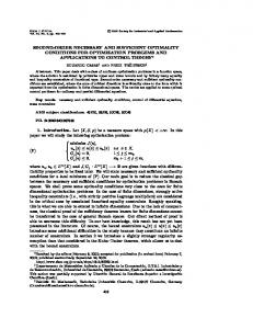
the discretized control problem with a large number N of grid points τi = i · tf /N, i = 0, 1, ..., N; cf. [2, 3]. We use the modeling language AMPL of Fourer et al. [6], the interior point optimization code IPOPT of W¨achter et al. [27] and the integration method of Heun. For N = 5000 grid points, the computed state, control and adjoint functions are displayed in Fig. 1. We find the following values for the switching time, functional value and some selected state and adjoint variables: t1 x1 (t1 ) x1 (tf ) ψ1 (0) ψ1 (t1 ) ψ1 (tf ) x1 (t)

= = = = = =

0.65691, 0.84924, 0., −7.8617, −8.4975, −8.72313,

J x2 (t1 ) x2 (tf ) ψ2 (0) ψ2 (t1 ) ψ2 (tf )

= = = = = =

x2 (t)

3

26.705, 0.226879, 0.574104, −4.70437, −3.2016, −9.13931.

(40)

1

0.9 2.5 0.8 2 0.7

1.5

0.6

0.5 1 0.4 0.5 0.3

0

0.2 0

v(t)

0.1

0.2

0.3

0.4

0.5

0.6

0.7

0.8

0

0.9

0.1

0.2

0.3

0.4

0.5

0.6

0.7

0.8

0.9

m(t)

3

4 2.5

3 2

1.5

2

1 1

0.5 0 0 0

ψ1 (t)

0.1

0.2

0.3

0.4

0.5

0.6

0.7

0.8

0.9

0

ψ2 (t)

-7.8

0.1

0.2

0.3

0.4

0.5

0.6

0.7

0.8

0.7

0.8

0.9

-3

-7.9 -4 -8 -5

-8.1 -8.2

-6 -8.3 -7 -8.4 -8.5

-8

-8.6 -9 -8.7 -8.8

-10 0

0.1

0.2

0.3

0.4

0.5

0.6

0.7

0.8

0.9

0

0.1

0.2

0.3

0.4

0.5

0.6

0.9

Figure 1: From above: state variables x1 (t) and x2 (t); control variables v(t) and m(t); adjoint variables ψ1 (t) and ψ2 (t). 17

Let us apply now the second-order sufficient conditions in Theorem 4.1. Observe first that the sufficiency theorem in Feichtinger and Hartl [5], p. 36, Satz 2.2, is not applicable here. The assumptions in this theorem require that the minimized Hamiltonian H min(t, x, ψ(t)) be convex in the state variable x = (x1 , x2 ). However, using the minimizing control v = −ψ1 x2 eρt /2r from (36), we obtain H min(t, x, ψ(t)) = −

eρt ψ1 (t)2 x22 + L(x), 4r

where L(x) denotes a linear function in the variable x. Since ψ1 (t) 6= 0 for t ∈ [0, tf ], the minimized Hamiltonian is strictly concave in the variable x2 . Hence, the sufficiency theorem in [5], Satz 2.2, can not be used here. Now we compute the quantities needed in Theorem 4.1 and (28). The derivative of the switching function σ m (t) = e−ρt c + ψ2 (t)(1 − x2 (t)) in (37) is given by σ˙ m = −ρe−ρt c − ψ1 v(1 − x2 ) + ψα,

v = −ψ1 x2 eρt /2r .

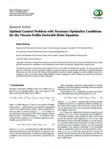
Inserting the values given in (40) we get D 1 (H) = −4σ˙ m (t1 ) = 27.028 > 0,

σ m (t) 6= 0 ∀ t 6= t1 .

Hence, the maintenance control m(·) is a strict bang-bang control; see Fig.2. σ m (t)

2.5

2

1.5

1

0.5

0

-0.5

-1

-1.5

-2 0

0.1

0.2

0.3

0.4

0.5

0.6

0.7

0.8

0.9

Figure 2: Switching function σ m (t). Now we evaluate the Riccati equation Q˙ = −Qfx − fx Q − Hxx + (Hxv + Qfv )(Hvv )−1 (Hvx + fv∗ Q) for the symmetric 2 × 2-matrix Q = fx =

0 v 0 −(α + m)

!

, fv =

q11 q12 q12 q22 x2 0 18

!

!

(41)

. Computing the expressions

, Hxx = 0, Hxv = (0, ψ1 ),

the matrix Riccati equation (41) yields the following ODE system: 2 2 ρt q˙11 = q11 x2 e /2r , q˙12 = q11 v − q12 (α + m) + eρt q11 x2 (ψ1 + q12 x2 ) , q˙22 = −2q12 v + 2q22 (α + m) + eρt (ψ1 + q12 x2 )2 /2r .

(42) (43) (44)

The equations (42) and (43) are homogeneous in the variables q11 and q12 . Hence, we can try to find a solution to the Riccati system with q11 (t) = q12 (t) ≡ 0 on [0, tf ]. Then (44) reduces to the linear equation q˙22 = 2q22 (α + m) + eρt ψ12 /2r .

(45)

Obviously, this linear equation has always a solution. The remaining difficulty is to satisfy the jump and boundary conditions in Theorem 4.1 (c) and (d). Instead of condition (c) we will verify conditions (c+) and (28) which are more convenient for the backward integration of (44). The boundary conditions in Theorem 4.1 (d) show that the initial value Q(0) can be chosen arbitrarily while the terminal condition imposes the sign condition q22 (tf ) ≤ 0, since x2 (tf ) is free. We shall take the boundary condition q22 (tf ) = 0 .

(46)

Using the computed values in (40), we solve the linear equation (45) with terminal condition (46). At the switching time t1 we obtain the value q22 (t1 ) = −1.5599 . Next, we evaluate the jump in the state and adjoint variables and will check conditions (28). We get ˙ = (0, Mψ2 (t1 )) , ([x] ˙ 1 )T = (0, M(1 − x2 (t1 )), [ψ] which yield the quantities q1+ = = b1+ = = =

˙ 1 = (0, M(1 − x2 (t1 ))q22 (t1 +) − Mψ2 (t1 ) ([x˙ 1 ]T Q1+ − [ψ] (0, 8.2439), D 1 (H) + (q1+ )[x˙ 1 ] D 1 (H) + M 2 ((1 − x2 (t1 )q22 (t1 +) − ψ2 (t1 ))ψ2 (t1 ) 27.028 + 133.55 = 165.58 > 0 .

Then the jump condition in (28), 1

−1

T

[Q] = (b1+ ) (q1+ ) (q1+ ) =

0 0 0 [q22 ]1

!

,

reduces to a jump condition for q22 (t) at t1 . However, we do not need to evaluate this jump condition explicitly because the linear equation (45) has a solution regardless of the value q22 (t1 −). Hence, we conclude from Theorem 4.1 that the numerical solution characterized by (40) and displayed in Fig. 1 provides a strict bounded–strong minimum. 19

6

Acknowledgement

We are indebted to Kazimierz Malanowski for helpful comments.

References [1] Agrachev, A.A., Stefani, G. and Zezza, P.L., Strong optimality for a bang–bang trajectory, SIAM J. Control and Optimization, 41 , 9911014 (2002). [2] Betts, J.T., Practical Methods for Optimal Control Using Nonlinear Programming. Advances in Design and Control, SIAM, Philadelphia, 2001. ¨skens C. and Maurer H., SQP–methods for solving optimal control [3] Bu problems with control and state constraints: adjoint variables, sensitivity analysis and real–time control. J. of Computational and Applied Mathematics, 120, pp. 85–108 (2000). [4] Cho, D.I., Abad, P.L., and Parlar, M., Optimal production and maintenance decisions when a system experiences age-dependent deterioration. Optimal Control Applic.and Methods, 14, pp. 153–167 (1993). [5] Feichtinger, G. and Hartl. R.F., Optimale Kontrolle ¨okonomischer Prozesse. de Gruyter Verlag, Berlin, 1986. [6] Fourer, R., Gay, D.M., and Kernighan, B.W., AMPL: A Modeling Language for Mathematical Programming. Duxbury Press, Brooks-Cole Publishing Company, 1993. [7] Hestens, M., Calculus of Variations and Optimal Control Theory, John Wiley, New York, 1966. [8] Malanowski, K., Stability and sensitivity analysis for optimal control problems with control–state constraints, Dissertationes Mathematicae, Polska Akademia Nauk, Instytut Matematyczny, 2001. [9] Maurer, H., First and second order sufficient optimality conditions in mathematical programming and optimal control, Mathematical Programming Study, 14, pp. 163–177 (1981). [10] Maurer, H., Kim, J.-H.R., and G. Vossen, G., On a state– constrained control problem in optimal production and maintenance, in: Optimal Control and Dynamic Games, Applications in Finance, Management Science and Economics, C. Deissenberg, R.F. Hartl, eds., pp. 289–308, Springer Verlag, 2005. 20

[11] Maurer, H. and Oberle, H.J., Second order sufficient conditions for optimal control problems with free final time: The Riccati approach, SIAM J. Control and Optimization, 41, pp. 380–403 (2002). [12] Maurer, H. and Osmolovskii, N.P., Second order sufficient conditions for time optimal bang–bang control problems SIAM J. Control and Optimization, 42, pp. 2239–2263 (2004). [13] Maurer, H. and Osmolovskii, N.P., Second order optimality conditions for bang–bang control problems, Control and Cybernetics, 32, No 3, pp. 555-584 (2003). [14] Maurer, H., and Pickenhain, S., Second-order sufficient conditions for control problems with mixed control-state constraints, Journal of Optimization Theory and Applications, 86, pp. 649-667 (1995). [15] Milyutin, A.A. and Osmolovskii, N.P. , Calculus of Variations and Optimal Control, Translations of Mathematical Monographs, Vol. 180, American Mathematical Society, Providence, 1998. [16] Oberle, H.J. and Taubert, K., Existence and multiple solutions of the minimum-fuel orbit transfer problem, J. Optimization Theory and Applications, 95, pp. 243–262 (1997). [17] Osmolovskii, N.P. , High-order necessary and sufficient conditions for Pontryagin and bounded-strong minima in the optimal control problems, Dokl. Akad. Nauk SSSR, Ser. Cybernetics and Control Theory 303, 1052– 1056 (1988), English transl., Sov. Phys. Dokl., 33, No. 12, 883–885 (1988). [18] Osmolovskii, N.P., Quadratic conditions for nonsingular extremals in optimal control (A theoretical treatment), Russian J. of Mathematical Physics, 2, pp. 487–516 (1995). [19] Osmolovskii, N.P., Second order conditions for broken extremal. In: Calculus of variations and optimal control (Technion 1998), A. Ioffe, S. Reich and I. Shafir, eds., Chapman and Hall/CRC, Boca Raton, Florida, 198–216 (2000). [20] Osmolovskii, N.P., Second-order sufficient conditions for an extremum in optimal control, Control and Cybernetics, 31, No 3, pp. 803–831 (2002). [21] Osmolovskii, N.P., Quadratic optimality conditions for broken extremals in the general problem of calculus of variations, Journal of Math. Science, 123, No. 3, pp. 3987–4122 (2004).

21

[22] Osmolovskii, N.P. and Lempio, F., Jacobi–type conditions and Riccati equation for broken extremal, Journal of Math. Science, 100, No.5, pp. 2572–2592 (2000). [23] Osmolovskii, N.P. and Lempio, F., Transformation of quadratic forms to perfect squares for broken extremals, Journal of Set Valued Analysis, 10, pp. 209–232 (2002). [24] Osmolovskii, N.P. and Maurer, H., Equivalence of second order optimality conditions for bang-bang control problems. Part 1: Main results, Control and Cybernetics, 34, 2005, pp 927–950; Part 2: Proofs, variational derivatives and representations, Control and Cybernetics 36, 2007, pp 5–45. [25] Pontryagin, L.S., Boltyanski, V.G., Gramkrelidze, R.V., and Miscenko, E.F., The Mathematical Theory of Optimal Processes, Fitzmatgiz, Moscow; English translation: Pergamon Press, New York, 1964. [26] Rosendahl, R., Second Order Sufficient conditions for space-travel optimal control problems, Talk presented at the 23rd IFIP TC7 Conference on Systems Modelling and Optimization, July 2007, Cracow, Poland. ¨chter, A, et al., http://projects.coin-or.org/Ipopt [27] Wa [28] Zeidan, V., The Riccati equation for optimal control problems with mixed state control problems: necessity and sufficiency, SIAM Journal on Control and Optimization, 32, pp. 1297-1321 (1994).

22