Secondary-Storage Confidence Computation for Conjunctive Queries ...

Secondary-Storage Confidence Computation for Conjunctive Queries with Inequalities Dan Olteanu and Jiewen Huang Computing Laboratory, Oxford University, Oxford, OX1 3QD, UK {dan.olteanu,jiewen.huang}@comlab.ox.ac.uk

ABSTRACT This paper investigates the problem of efficiently computing the confidences of distinct tuples in the answers to conjunctive queries with inequalities ( 1, are obtained for free, once we computed the OBDD for fx1 . Example 4.3. Example 2.2 discusses how the lineage of the query Q5 above on the database (R, T ′ ) of Figure 3 can be compiled into an OBDD of linear size. We next discuss the case of the query Q6 : Q6 :-R′ (E, F ), T (D), T ′ (G, H), E < D < H.

Consider the probabilistic database (R′ , T, T ′ ) of Figure 3, where the variables of T ′ are z1 , z2 , z3 instead of y1 , y2 , y3 . The lineage of the answer to query Q6 on this database is x1 [y1 (z1 + z2 + z3 )+ x2 [ x3 [

y2 (z2 + z3 )+y3 z3 ]+ y2 (z2 + z3 )+y3 z3 ]+ y3 z3 ].

We can check that the inclusion relation holds between the cofactors of variables xi : fx1 ⊃ fx2 ⊃ fx3 . The same applies to the cofactors of variables yi . Although it is not here the case, in general the inclusion may not be strict. That is, two variables may have the same cofactor. For instance, if two tuples of R′ have the same E-value, then their variables have the same cofactors. The above lineage can be easily compiled into an OBDD of size linear in the number of variables in the lineage, see Figure 4(right). We first eliminate the variables x1 , x2 , x3 , and then reduce the cofactor fx1 to fx2 by eliminating variable y1 , and then to fx3 by eliminating y2 . The variable

order of our OBDD has then y1 before y2 before y3 . Note that the variables y1 and z1 are those that occur in fx1 and not in fx2 , although to get from fx1 to fx2 we only need to set y1 to false. The same applies to variables y2 and z2 . After removing y1 , the branch y1 = 0 points to fx2 , and the other branch y1 = 1 points to z1 +z2 +z3 . After removing y2 , we point to fx3 and to z2 + z3 . In case of y3 , we point to 0 and to z3 . The sums z1 + z2 + z3 , z2 + z3 , and z3 can be represented linearly under the variable order z1 z2 z3 , because (z1 + z2 + z3 ) ⊃ (z2 + z3 ) ⊃ z3 . 2 We can now summarize our results on inequality paths. Theorem 4.4. Let φ be the lineage of any IQ query with inequality paths on any tuple-independent database. Then, we can compute a variable order π for φ in time O(|φ| · log |φ|) under which the OBDD (φ, π) has size bounded in |V ars(φ)| and can be computed in time O(|V ars(φ)|). We thus obtain linear-size OBDDs for lineage whose size can be exponential in the query size. This result supports our choice of OBDDs as a data structure that can naturally capture the regularity in the lineage of tractable queries.

4.3 Queries with Inequality Trees We generalize the results of Section 4.2 to the case of inequality trees. Examples of such IQ queries are: Q7 :-R′ (E, F ), T (D), S(B, C), E < D, E < C and Q8 :-R′ (E, F ), T (D), S(B, C), T ′ (G, H), E < D, E < C < H.

The lineage of queries with inequality paths and of queries with inequality trees have different structures. We explain using the lineage of query Q7 , where we assume that table R′ has variables x1 , . . . , xn , table T has variables y1 , . . . , ym , and table S has variables z1 , . . . , zk , and that the tables are already sorted on their attributes involved in inequalities. We will later exemplify with a concrete database. As for inequality paths, the lineage can be expressed as Σi xi fxi , but now each cofactor fxi of xi is a product of a sum of variables yi and of a sum of variables zj . In contrast, for an inequality path E < D < C, a cofactor fxi would be a sum of variables yj , each with a cofactor fyj that is a sum of z-variables. The inclusion relation still holds on the cofactors of variables xi : fx1 ⊇ . . . ⊇ fxn , and we can thus obtain any fxi+1 from fxi by setting to false variables that occur in fxi and not in fxi+1 . These variables can be both y-variables and z-variables; to compare, in the case of inequality paths, the elimination variables need only be y-variables. The inclusion relation holds because of the transitivity of inequality: If we consider any two E-values e1 and e2 such that e1 < e2 , the tuples of T and S joined with e2 are necessarily also joined with e1 . The inclusion relation holds even if the variables yi or zj have themselves further cofactors due to further inequalities, provided the cofactors of variables yi are independent from the cofactors of variables zj . Example 4.5. Consider the database consisting of tables R′ , T , and S of Figure 3, where we add variables z1 to z5 to the tuples of table S. The lineage of query Q7 is x1 (y1 + y2 + y3 )(z1 + z3 + z2 + z5 + z4 )+ x2 (y2 + y3 )(z2 + z5 + z4 )+ x3 (y3 )(z4 ).

Assumptions: Input tree is the query’s inequality tree and has n nodes. Input t is the query answer before confidence computation. For each node in tree, tuples in t have its column X involved in inequalities and the variable column V of its table. processLineage(IneqTree tree, Tuples t) { assign indices {1,2,...,n} to each node in tree according to its position in a depth-first preorder traversal; sort t on (X1 desc, V1 , ..., Xn desc, Vn ), where Xi and Vi are from the table of node with index i in tree; let t′ be πV1 ,V2 ,...,Vn (sorted t); crtTuple = first tuple in t′ ; varOrder = NULL; foreach node no of tree do { no.firstVar = crtTuple[Vno.index ]; no.latestVarInVO = NULL; no.varToInsert = crtTuple[Vno.index ]; } { nextTuple = next tuple in t′ ; find minimal i such that crtTuple[Vi ] 6= nextTuple[Vi ]; foreach node no of tree with index from n to i do { if (no.varToInsert 6= NULL) { insert no.varToInsert at the beginning of varOrder; no.latestVarInVO = no.varToInsert; no.varToInsert = NULL; } if (crtTuple[Vno.index ] 6= nextTuple[Vno.index ] AND crtTuple[Vno.index ] = no.latestVarInVO AND nextTuple[Vno.index ] 6= no.firstVar) no.varToInsert = nextTuple[Vno.index ]; } crtTuple = nextTuple; } do while (crtTuple 6= NULL); }

Figure 8: Incremental computation of variable orders for IQ queries with inequality trees. It indeed holds that fx1 ⊃ fx2 ⊃ fx3 . We can transform fx1 into fx2 by eliminating in any order y1 and (z1 , z3 ). We then transform fx2 into fx3 by eliminating y2 and (z2 , z5 ). According to the elimination order constraints imposed by transformations on cofactors, an interesting variable order is x1 x2 x3 y1 z1 z3 y2 z2 z5 y3 z4 . Figure 12 gives a fragment of the OBDD for this lineage in case x1 is set to false. As we can see, each variable xi has one OBDD node, and each variable yi or zi has up to two OBDD nodes. This is because the lineage states no correlation between the truth assignments of any pair of variables yi and zj . Hence, in case we eliminate, say, yi , nodes for variable zj can occur under both branches of the yi node. There are, of course, other variable orders that do not violate the constraints. For instance, we could eliminate y1 z1 z3 after x1 and before x2 , and similarly for y2 z2 z5 : We then obtain x1 y1 z1 z3 x2 y2 z2 z5 x3 y3 z4 . The reverse of any such order also induces succinct OBDDs. 2 As in the case of inequality paths, we can always find a variable order for the cofactor fx1 such that its OBDD already includes the OBDDs of the cofactors fxi of all variables xi where i > 1. This order must agree with constraints on variable elimination orders imposed by transforming fxi

into fxi+1 , for all i ≥ 1. Example 4.5 (above) shows how such orders can be computed for a reasonably small lineage. For the case of general IQ queries with inequality trees, one can use the algorithm given in Figure 8. This algorithm works on a relational encoding of the lineage (as produced by queries) and, after sorting the lineage, it only needs one scan. It uses the inequality tree to rediscover the structure of the lineage. Because of the maxone property of the conjunction of inequalities, there is one table for each node in the inequality tree. Each node in the inequality tree contains four fields: index, firstVar, latestVarInVO and varToInsert. The field index serves as an identifier of the node, whereas the other three fields store information related to the variables from the corresponding table. The field firstVar stores the first variable from the table that has been inserted into the variable order. It is set as the variable in the first tuple after sorting and does not change afterwards. The field latestVarInVO stores the latest variable from the table inserted into the variable order, and the field varToInsert stores the new variable encountered in the input tuples but not yet inserted into the variable order. The variable order construction is triggered by the changes in the variable columns between two consecutive tuples. The sorting is crucial to the algorithm, as it orders the lineage such that the cofactor fxi+1 is encountered before fxi in one scan of the lineage. We thus compute the variable order for fxi+1 before computing it for fxi . Because the OBDD for fxi+1 represents a subgraph of the OBDD for fxi , the variable order for fxi+1 is a suffix of the variable order for fxi . A key challenge here is to identify a variable that has not been inserted into the variable order. An inefficient approach is to look it up in the variable order constructed so far. This can be solved more efficiently, however, by only using firstVar and latestVarInVO. Due to sorting and the inclusion property between the cofactors of variables from the same table, all variables encountered after firstVar and before latestVarInVO while scanning the cofactor of a variable have already been inserted into the variable order. After scanning the cofactor of latestVarInVO, if the next variable in the same column of the next tuple is not firstVar, this indicates that this variable has not been encountered and we store it in varToInsert. Example 4.6. Consider the lineage of Example 4.5. We scan it in the order x3 y3 z4 , x2 y3 z4 , x2 y3 z5 , x2 y3 z2 and so on. Initially, the first tuple is read and firstVar and varToInsert are set to the variables in this tuple. On processing the second tuple, a change is found on the first variable column, all varToInsert values stored in the nodes are inserted into the variable order and obtain x3 y3 z4 . The fields latestVarInVO of nodes for query variables E, D, and C are also updated accordingly to x3 , y3 , and z4 respectively. On reading the third tuple, a change in the third variable column is detected and varToInsert is updated to z5 . On reading the fourth tuple, a change is again detected in the third variable column and z5 is inserted into the variable order. We thus obtain the order z5 x3 y3 z4 , In addition, latestVarInVO is updated to z5 and varToInsert is set to z2 . The final variable order is x1 y1 z1 z3 x2 y2 z2 z5 x3 y3 z4 . 2 Under such variable orders, the OBDDs can have several nodes for the same variable. As pointed out in Example 4.5 for the lineage of query Q7 , this is because there is no con-

straint between variables yi and zj : Setting a variable yi to true or false does not influence the truth assignment of a variable zj . We next analyze the maximum number of OBDD nodes for a variable in case of an inequality tree consisting of a parent with n children: Q8 :-R(X), S1 (Y1 ), . . . , Sn (Yn ), X < Y1 , . . . , X < Yn i , where R and Si have variables x1 , . . . , xm , and y1i , . . . , ym i

Figure 9: Partial OBDD used in Example 4.9.

n

respectively. The lineage is Σi xi ( Π fxi (y j )), where each j=1

fxi (·) is a sum of variables from the same table. We know that the OBDD obtained by compiling the cofactor of x1 contains the OBDDs for the cofactors of all other xi (i > 1), under the constraint that the variable order transforms one cofactor into the next. This means that, in order to compile the cofactor of x1 , we need to use an intertwined elimination of variables y 1 to y n . Consider we want to count the number of OBDD nodes for variable yji . The OBDD nodes that can point to yji nodes represent expressions that can have any of the form

4.4 Queries with Inequality Graphs

from each variable group, can point to yji -nodes only if the sum s(y i ) contains the variable yji and all its preceding variables y i are set to false. Then, again, there is one path from the root to that node that follows the false edges of the eliminated variables y i , and hence one yji -node to point to. In case of expression forms, where some of the sums are missing, we use the same argument: precisely one variable from each of these sums is set to true, and there is a single path from the root to the node representing that expression, and hence one yji -node to point to. This result can be generalized to arbitrary inequality trees.

We next consider IQ queries with inequality graphs. In case the inequality graph is cyclic, then the query is unsatisfiable, as an inequality of the form A < B < A can be derived from the transtivity of inequality. An inequality graph with several unconnected components means that the query is a product of independent subqueries, one subquery per unconnected component. This case is approached as described in Section 4.1. In case of connected inequality graphs, the structure of the lineage for such queries differs from that of inequality trees. Our approach is to simplify the inequality graph by eliminating all its sink nodes, i.e., all nodes that have more than one incoming edge. After elimination, we are left with an inequality tree, which can be processed as presented in Section 4.3, or with several unconnected inequality trees, which can then be processed independently. The elimination of a node from an inequality graph corresponds to the construction of a variable order where all (random) variables of the table corresponding to that node occur together and before the variables of other tables. The order of these variables has to follow the inclusion of their cofactors such that the variable xi+1 occurs before xi if fxi ⊂ fxi+1 . This order is the order of the indices of variables xi , assuming the variables xi are initially sorted according to the values of the attribute mapped to that inequality node. If several nodes in the inequality graph need to be eliminated, then their elimination order is irrelevant. In case of two such nodes, say with corresponding tables R1 and R2 , their elimination leads to variable orders starting with all the variables xn , . . . , x1 of the table R1 , followed by all the variables ym , . . . , y1 of the table R2 , and finally completed with the variables from the remaining tables. Because the elimination of a variable from R1 may not affect the truth of any variable from R2 , the OBDD fragment constructed under the variable order xn . . . x1 ym . . . y1 can have size n · m: for each variable xi , the same variable yj can occur under both of its branches. (Note again that variables xl with l < i cannot occur under the positive branch of xi because their cofactors are subsumed by the cofactor of xi .) This property generalizes to k inequality sink nodes to be removed from an inequality graph.

Theorem 4.7. Let φ be the lineage of any IQ query with inequality tree t on any tuple-independent database. Then, we can compute a variable order π for φ in time O(|φ| · log |φ|), under which the OBDD (φ, π) has size and can be computed in time O(2|t| · |V ars(φ)|).

Theorem 4.8. Let φ be the lineage of any IQ query on any tuple-independent database. Let g be the inequality graph, whose sink nodes correspond to tables T1 , . . . , Tk . Then, we can compute a variable order π for φ in time O(|φ| · log |φ|), under which the OBDD (φ, π) has size O(2|g|−k · |V ars(φ)| ·

l≤n

s(y i ) Π s(y k )) or simply s(y i ), where the functions s(y k ) k=1,6=i

k stand for sums over variables y1k , . . . , ym . All such expresk sions necessarily contain a sum over variables y i , which includes yji ; otherwise, their OBDD nodes cannot point to yji -nodes. The number of distinct forms is exponential in n (more precisely, half the size of the powerset of {1, . . . , n}; those without s(y i ) are dropped). Interestingly, there can be precisely one OBDD node for each of these forms that point to an yji -node. This means that the number of yji nodes is in the order of O(2n ). We explain this for three of the possible forms. A node representing an expression s(y i ) can point to an yji -node if, according to our elimination order, the variables y i preceding yji are all dropped, and precisely one variable from the remaining variable groups is set to true. Then, there is a single path from the OBDD root to the node for the expression s(y i ), following the true and false edges of the eliminated variables, and hence only one yji -node to point to. A node representing an expression n

s(y i ) Π s(y k )), which is a product of sums of variables k=1,6=i

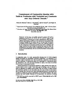
The OBDD for φ does not need all O(2|t| ) nodes for each variable. Figure 12 shows two OBDDs for a fragment of the lineage of query Q7 of Example 4.5, one as constructed by our algorithm (right), and a reduced version of it (left).

k

Π (|V arsTi (φ)|)).

i=1

We next exemplify with an inequality graph that has one sink node.

OBDD Node: probability p, bool vector bv, children hi from the solid edge and lo from the dotted edge Level: a vector of OBDD Nodes nodes, index of the inequality tree node whose table contains the variables at this level index n: the number of nodes in the inequality tree obdd levels: Level[n + 1]

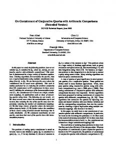
Figure 10: Data structures used by the algorithm of Figure 11. Example 4.9. Let the IQ query with inequality graph Q9 :-R(A), T (D), R′ (E, F ), T ′ (G, H), A < E, D < E, D < G

on the database (R, R′ , T, T ′ ) of Figure 3, with the modification that R′ has variables z1 , z2 , z3 and T ′ has variables u1 , u2 , u3 . Its inequality graph has the sink node labeled E corresponding to the table R′ . The lineage is x1 y1 (z2 + z3 )(u2 + u3 ) + x1 y2 z3 u3 + x2 y1 z3 (u2 + u3 ) + x2 y2 z3 u3 + x 3 y2 z 3 u3 .

We remove from the inequality graph the sink node E and obtain two unconnected graphs: one isolated node A, and a path D → G. This removal operation corresponds to the elimination of variables z3 and z2 from the lineage. The formulas remaining after these variable eliminations can then be (separately) compiled as for unconnected graphs. The partial OBDD structure obtained by eliminating the variables z3 and z2 is shown in Figure 9. We also show the OBDD for the cofactor of z3 in Figure 7(right). 2

5.

CONFIDENCE COMPUTATION IN SECONDARY STORAGE

This section introduces a secondary-storage algorithm for confidence computation for IQ queries with inequality trees. For queries with arbitrary inequality graphs, we follow the node elimination algorithm given in Section 4.4, which transforms arbitrary inequality graphs into (possibly unconnected) trees. We then apply the algorithm of this section. This algorithm is in essence our algorithm for incremental computation of variable orders for queries with inequality trees given in Figure 8 of Section 4. An important property of this algorithm is that it does not require the OBDD to be materialized before it starts the computation. The key ideas are (1) to construct the OBDD levelwise, where a level consists of the OBDD nodes for one variable in the input lineage, and (2) to keep in memory only the necessary OBDD levels. Similar to the algorithm that computes variable orders, this confidence computation algorithm needs only one scan over the sorted lineage to compute its probability. The algorithm is given in Figure 11 and uses data structures described in Figure 10: The code in the topmost box should replace the inner box of the algorithm for variable order computation given in Figure 8. Let a query Q with inequality tree t of size n and let φ be the lineage of Q on some database. As discussed in Section 4.3, each variable in φ can have up to 2|t| OBDD nodes, which form a complete OBDD level. When a new variable is encountered, instead of adding it to the variable order, we construct a new level of nodes in the OBDD for this variable.

Code to replace the inner box in Figure 8: add level(i, no.varToInsert.prob); Initialization: create Level L; L.nodes = OBDD Node[2n ]; L.index = 0; foreach OBDD Node no in L.nodes do { no.bv = distinct bool vector of size n; if (any value in no.bv is false) no.p = 0; else no.p = 1; } insert L at beginning of obdd levels; add level(int i, Prob p) create Level L; L.nodes = OBDD Node[2n−1 ]; L.index = i; foreach OBBD node no in L.nodes do { no.bv = distinct bool vector of size n where bv[i] = false; no.lo = get node(no.bv, i, false); no.hi = get node(no.bv, i, true); no.p = p × no.hi.p + (1 − p) × no.lo.p; } remove L′ from obdd levels such that L′ .index = i; insert L at beginning of obdd levels; get node(bool vector bv, int i, bool is true) bv[i] = is true; crtLevel = the first Level in obdd levels; while(true) if (crtLevel.index = 0 OR (!bv[crtLevel.index] AND all ancestors set true(bv, crtLevel.index))) foreach OBDD node no in crtLevel.nodes do if (no.bv = bv) { bv[i] = false; return no; } else crtLevel = the next Level in obdd levels; all ancestors set true(bool vector bv, int i) foreach ancestor A of get ineqtree node with index(i) do if (!bv[A.index]) return false; return true;

Figure 11: Secondary-storage algorithm for confidence computation. The major challenge lies in how to connect the low and high edges of a node to the correct (lower) nodes in the levels kept in memory. Recall that every OBDD node represents a partial lineage obtained by eliminating variables at the upper OBDD levels. In an OBDD, none of the nodes represent the same formula. The formulas determine the connection between nodes from different levels. For instance, in Figure 12, the left and right nodes in the level of y3 represent formulas y3 z4 and y3 respectively. The formula at the leftmost node x3 is x3 y3 z4 , and hence the high edge of this node must point to y3 z4 and not to y3 . The formula can be, however, large and, instead of materializing it, we use a compact representation of it. This is possible due to the lineage structure imposed by the query and the chosen variable elimination order. Our compact representation is that of a Boolean vector of size n. A “true” value in this Boolean vector at position i indicates that a variable from the table with index i has been set to true. This means that the formula at that node does not contain further variables from the table with index i (property of OBDDs representing lineage of queries with inequality trees). The Boolean vectors act as the identifiers of the OBDD nodes so that the nodes from the level above can identify a potential child node among the ones at this level.

x2[FFF]

y2[FFF]

x2[FFT]

y2[FFT]

z2[FFF]

y2[TFF]

z2[FTF]

z5[TFF]

z5[FTF]

x3[FFT]

x3[FTF]

y3[TFF]

x2[FTT]

y2[TFT]

z2[TFF]

z5[FFF]

x3[FFF]

x2[FTF]

z2[TTF]

z5[TTF]

x3[FTT]

y3[TFT]

z4[TTF]

0

1

Left: Reduced OBDD used in Section 4. Right: Partially reduced OBDD as constructed by the algorithm of Section 5. Constant nodes are merged, and nodes z4 [FFF], z4 [FTF], z4 [TFF], y3 [FFT] and y3 [FFF] are removed for compactness (although the algorithm constructs them). Grey nodes form the equivalent reduced OBDD on the left. Figure 12: OBDDs for the lineage discussed in Example 4.5. The algorithm works as follows: We initially build a level of one constant node 1 and 2n − 1 constant nodes 0. Note that this construction does not lead to reduced OBDDs, but it is sufficient for our processing task. For every new variable encountered during the scan, we build a level of OBDD nodes, and for each such node find its high and low children nodes in the existing levels. The probability of a node can be computed only based on the probabilities of the nodes it points to. Therefore, the probability computation and the OBDD construction go in parallel. Instead of keeping all the levels of the OBDD in memory, our algorithm keeps only one level for every table in the condition tree t. As soon as a new level is built for a variable from a table, the old level for the variable from the same table is dropped if there is any. This is possible because of the following property of the OBDDs for queries with inequality trees: Let x1 and x2 be variables from the same relation and the level of x1 higher than the level of x2 . Then, no edge from levels above the level of x1 points to nodes in the level of x2 . This is due to the inclusion property between the cofactors in the lineage. The algoritm also exploits two properties of such OBDDs: • No OBDD node for a variable from a table is accessible via the high edge of an upper OBDD node for a variable from the same table. • Let a table R and its ancestors S1 , . . . , Sn in the inequality tree. Then, a path from the root to an OBDD node for a variable from R must follow the high edges of at least one node for a variable from each S1 , . . . , Sn . Both these properties are used in the outermost if-condition of the procedure get node in Figure 11. Example 5.1. We show how to compute the probability of the lineage of query Q7 of Example 4.5. Figure 12 shows a fragment of its OBDD. The inequality tree is of size 3. The number of constant nodes is thus 23 = 8 and of non-constant nodes per level is 22 = 4. The size of a Boolean vector is 3 and the corresponding inequality tree nodes of tables R′ , T and S are assigned indices 1, 2 and 3 respectively.

We build a level of eight constant nodes: Seven nodes with at least one false value (F) in the Boolean vector have probability 0 (they are merged into one in Figure 12) and the remaining one with [T,T,T] has probability 1. We then construct four nodes in the level for z4 . The corresponding Boolean vectors of the nodes are [T,T,F], [T,F,F], [F,T,F], and [F,F,F]. The value in all the vectors for the variables of table S is F because formulas of all nodes at this level contain variable z4 ; otherwise, elimination of z4 will be redundant. The first vector encodes a formula with variables only from S. The second vector encodes a formula with variables only from T and S, and so on. The outgoing edges of nodes z4 can only point to the only level below, which is made by constant nodes. For instance, the high and low edges of node with vector [T,T,F] point to nodes with [T,T,T] and [T,T,F] respectively, that is, to nodes 1 and 0 respectively. Hence, its probability is Pr(z4 )× 1 + Pr(z4 ) × 0 = Pr(z4 ). Consider that the level for variable y3 is already constructed similarly to the previous level (z4 ), and let us construct the level for x3 . We create four nodes with Boolean vectors [F,T,T], [F,T,F], [F,F,T], [F,F,F]. For the node with vector [F,F,F], since the corresponding value for relation R′ in the vector is F and the inequality tree node of R′ is the ancestor of those of S and T , its low edge cannot point to nodes in y3 and z4 levels, but instead points to constant node with vector[F,F,F], namely node 0. Its high edge points to the node with vector [T,F,F] in the level for y3 . Therefore, its probability is Pr(x3 ) × (node with vector [T,F,F] in y3 level).p + Pr(x3 ) × 0. Let us consider the final step. We construct the level for x1 . As the other non-constant node levels, it has four nodes. Since x1 is the first to be eliminated in the OBDD, the corresponding values for R′ , S, and T in the Boolean vector of the root should be F. Therefore, the probability of the lineage is given by the value p of the node with vector [F,F,F] in the level x1 and the other three nodes are redundant. Its probability is Pr(x1 )× (node with [T,F,F] in y1 level).p + Pr(x1 )× (node with [F,F,F] in x2 level).p. 2

1 2

3

4 5 6

select conf() from orders, lineitem where o orderkey = l orderkey and o orderdate > l shipdate - 3; select conf() from customer, orders, lineitem where c custkey = o custkey and o orderkey = l orderkey and c registrationdate + 30 < o orderdate and o orderdate + 100 < l shipdate; select conf() from customer, orders, lineitem where c custkey = o custkey and o orderkey = l orderkey and c registrationdate + 30 < o orderdate and c registrationdate + 100 < l receiptdate; select conf() from part, lineitem where p partkey = l partkey and l extendedprice / l quantity ≤ p retailprice; select conf() from orders, lineitem where o orderdate < l shipdate and l quantity > 49 and o totalprice > 450000; select s nationkey, conf() from supplier, customer where s acctbal < c acctbal and s nationkey = c nationkey and s acctbal > 9000 group by s nationkey;

Figure 13: Queries used in the experiments.

6.

EXPERIMENTS

Our experiments are focused on three key issues: scalability, comparison with existing state-of-the-art algorithms, and comparison with “plain” querying where we replaced confidence computation by a simple aggregation (counting). The findings suggest that our confidence computation technique scales very well: We report on wall-clock times around 200 seconds to compute the probability of query lineage of up to 20 million clauses. When compared with existing confidence computation algorithms, our technique outperforms them by up to two orders of magnitude in cases when the competitors need less than the allocated time budget of 20 minutes. We also found that lineage sorting has the lion’s share of the time needed to compute the distinct answer tuples and their confidences. Prototype. We implemented our secondary-storage algorithm and integrated it into SPROUT [15]. SPROUT is a scalable query engine for probabilistic databases that extends the query engine of PostgreSQL with a new physical aggregation operator for confidence computation. TPC-H Data. We generated tuple-independent databases from deterministic databases produced using TPC-H 2.8.0. We added to the table Customer a c_registrationdate column and set all of its fields to 1993-12-01. This value was chosen so that the inequality predicates in our queries are moderately selective: 1993-12-01