Segmentation for Hyperspectral Images with Priors

Segmentation for Hyperspectral Images with Priors Jian Ye, Todd Wittman, Xavier Bresson, Stanley Osher Department of Mathematics, University of California, Los Angeles, CA 90095

Abstract. In this paper, we extend the Chan-Vese model for image segmentation in [1] to hyperspectral image segmentation with shape and signal priors. The use of the Split Bregman algorithm makes our method very efficient compared to other existing segmentation methods incorporating priors. We demonstrate our results on aerial hyperspectral images.

1

Introduction

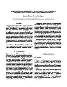
A hyperspectral image is a high-dimensional image set that typically consists of 100-200 image channels. Each channel is a grayscale image that indicates the spectral response to a particular frequency in the electromagnetic spectrum. These frequencies usually include the visible spectrum of light, but most of the channels are focused in the infrared range. This allows a hyperspectral image to reveal features that are not visible in a standard color image. Each pixel in the image will have a spectral response vector that is the high-dimensional equivalent of the pixel’s “color”. Certain materials have a characteristic spectral signature that can be used to identify pixels containing that material. In an aerial hyperspectral scene an analyst could, for example, locate manmade materials or distinguish healthy vs. dead vegetation. For this reason, there is great interest in developing fast detection methods in hyperspectral imaging for applications such as aerial surveillance, mineral and agricultural surveys, chemical analysis, and medical imaging. Unfortunately, due to the high dimensional complexity of the data, it is difficult to create accurate image segmentation algorithms for hyperspectral imagery. To improve the segmentation results, prior knowledge about the target objects can be incorporated into the segmentation model. In the spectral domain, a spectral prior is a vector specifying a target spectral signature that the pixels in the segmented object should contain. For example, one could specify the spectral signature of a particular mineral or type of biological tissue. This signature could be obtained from a spectral library or selecting a pixel from the image that is known to contain the desired material. In the spatial domain, a shape prior is a template binary image describing the outline of the desired targets. For example, in an aerial image one might use an airplane silhouette for automatically locating airplanes or in medical imaging one might enforce circular shapes to locate blood cells. An illustration of these two types of priors is shown in Fig. 1.

2

Jian Ye, Todd Wittman, Xavier Bresson, Stanley Osher

Fig. 1. Example priors. Left: Shape prior for outline of an airplane. Right: Signal prior for the hyperspectral signature of metal found in used in aircraft.

Image segmentation using shape priors has had great developments in recent years. Cremers, Osher and Soatto[2] incorporated statistical shape priors into image segmentation with the help of the level set representation. Their prior is based on an extension of classical kernel density estimators to the level set domain. They also propose an intrinsic registration of the evolving level set function which induces an invariance of the proposed shape energy with respect to translation. Using the level set representation, several other methods[3–5] have also been developed in recent years. Bresson et.al.[4] extended the work of Chen et. al.[6] by integrating the statistical shape model of Leventon et. al.[7]. They propose the following energy functional for a level set function φ and grayscale image I:

F (φ, xT , xpca ) =

Z

{gǫ (|∇I(x)|) + β φˆ2 (gxT (x), xpca )}δ(φ)|∇φ|dΩ

(1)

Ω

where gǫ is a decreasing function vanishing at infinity. The first term is the geodesic active contours classical functional which detects boundaries with the edge detector gǫ . The second term measures the similarity of the shape to the ˆ T , xpca ). zero level set of φ(x Later on, Bresson et. al.[5] used the boundary information and shape prior driven by the Mumford-Shah functional to perform the segmentation. They propose the following functional:

F = βs Fshape (C, xpca , xT )+βb Fboundary (C)+βr Fregion (xpca , xT , uin , uout ). (2)

Segmentation for Hyperspectral Images with Priors

3

with Fshape =

I

1

I

1

φˆ2 (xpca , hxT (C(q)))|C ′ (q)|dq,

(3)

g(|∇I(C(q))|)|C ′ (q)|dq,

(4)

0

Fboundary =

0

Fregion =

Z

+

Z

Ωin (xpca ,xT )

(|I − µin |2 + µ|∇uin |2 )dΩ

Ωout (xpca ,xT )

(|I − µout |2 + µ|∇uout |2 )dΩ

(5)

In the above functional, the first term is based on a shape model which constrains the active contour to retain a shape of interest. The second term detects object boundaries from image gradients. The third term globally drives the shape prior and the active contour towards a homogeneous intensity region. Recently, Cremers et.al.[8] used a binary representation of the shapes and formulated the problem as a convex functional with respect to deformations, under mild regularity assumptions. They proposed the following energy functional

Ei (q) =

Z

f (x)q(x)dx +

Z

g(x)(1 − q(x))dx +

Z

h(x)|∇q(x)|dx

(6)

The above first two terms are the integrals of f and g over the inside and outside of the shape, while the last term is the weighted Total Variation norm[9]. Ketut et.al.[10] applied the technique of graph cuts to improve the algorithm runtime. In this paper, we further improve the speed of the segmentation model with shape priors by using the Split Bregman method[10–13], a recent optimization technique which has its roots in works such as [14–16]. Also, we adapt the model to the hyperspectral images by the use of spectral angle distance and a signal prior.

2

Image Segmentation with Shape Priors

Variational methods have been widely used for the image segmentation problem. One of the most successful segmentation models is the Active Contour Without Edge(ACWE) model proposed by Chan and Vese[1]. To segment a grayscale image u0 with a curve C, the authors proposed the following energy functional: F (c+ , c− , C) = µ · Length(C) + λ+ + λ−

Z

inside(C) Z

|u0 (x, y) − c+ |2 dxdy

outside(C)

|u0 (x, y) − c− |2 dxdy

(7)

4


where Length(C) is the length of the curve C and c+ and c− denote the average intensity value inside and outside the curve, respectively. This is a two-phase version of the Mumford-Shah model. The idea is that C will be a smooth minimal length curve that divides the image into two regions that are as close as possible to being homogeneous. Later on, Chan and Vese extended the model to vector valued images[17] as Z N 1 X + λi |u0 (x, y) − c+ |2 dxdy (8) N i=1 inside(C) Z N 1 X − λ |u0 (x, y) − c− |2 dxdy + N i=1 i outside(C)

F (c+ , c− , C) = µ · Length(C) +

+ + − + − where λ+ i and λi are parameters for each channel, c = (c1 , ..., cN ) and c = − − (c1 , ..., cN ) are two unknown constant vectors. Chan et.al. proposed a convexification of Chan-Vese model in[18]. Analogously, we can convexify the vectorial version of Chan-Vese model in this way: Z E(u) = min g|∇u| + µ < u, r > (9) 0≤u≤1

PN

2 2 where r = N1 i=1 [(c1 − fi ) − (c2 − fi ) ] and fi is i-th band of the hyperspectral image with a total of N bands. In order to constrain the geometry shape of the resulting object, we want to minimize the area difference of shape prior and resulting object up to an affine transformation. The proposed energy functional is as follows: Z E(u) = min g|∇u| + µ < u, r > +α|u − w| (10) 0≤u≤1,xT

where w = hxT (w0 ), w0 is the shape prior, and hxT is a geometric transformation parameterized by xT . The above equation can be solved in an iterative way. It consists of following two steps. Step 1: Update u. Fix the prior w and its associated pose parameters xT and update u by using the fast Split Bregman algorithm. To apply the Split Bregman algorithm, we make the substitutions d1 = ∇u = (ux , uy )τ , d2 = u − w, d = (dτ1 , d2 )τ , F (u) = (ux , uy , u − w)τ . To approximately enforce these equality constraints, we add two quadratic penalty functions. This gives rise to the unconstrained problem

(u∗ , d∗ ) = arg min |d1 |g + α|d2 | + µ < u, r > + 0≤u≤1,d

+

λ2 ||d2 − (u − w)||22 2

λ1 ||d1 − ∇u||22 2 (11)


5

Then we apply Bregman iteration to the unconstrained problem(11). This results in the following sequence of optimization problems: (uk+1 , dk+1 ) = arg min |d1 |g + α|d2 | + µ < u, r > 0≤u≤1,d

λ1 λ2 ||d1 − ∇u − bk1 ||22 + ||d2 − (u − w) − bk2 ||22 2 2 = bk1 + (∇uk − dk1 ) = bk2 + (uk − w − dk2 )

(12)

+

bk+1 1 bk+1 2

(13)

where u can be solved by Gauss-Seidel iteration and d can be solved by shrinkage. The whole algorithm for solving for u is as follows: 1: while kuk+1 − uk k > ǫ do 2: Define rk = (ck1 − f )2 − (ck2 − f )2 3: uk+1 = GSGCS (rk , dk , bk ) 4: dk+1 = shrinkg (∇uk+1 + bk , λ) 5: bk+1 = bk + ∇uk+1 − dk+1 6: Find Ωk = {x : uk (x) > µ} R R f dx f dx Ωc Ω 7: Update ck+1 = Rk , and ck+1 = Rk 1 2 Ωk

dx

Ωc k

8: end while

dx

Step 2: , fix u and update xT . The parameters we consider for affine transformations are rotation θ, translation T and scaling s. For affine transformations, we can express xold = x− D = sA(x − c) + T . Here D is the displacement vector, A is a rotation matrix, T is the translation vector and s is the scaling factor. A is a function of the rotation angle θ.

A(θ) =

h cos θ − sin θ i sin θ cos θ

(14)

The derivative of the matrix A is

Aθ (θ) =

h − sin θ − cos θ i cos θ − sin θ

(15)

If we fix u, then the original optimization problem(10) becomes E(xT ) = α|u − w| = α|u − w0 (sA(x − c) + T )|

(16)

6


By the calculus of variations, we have Tt = −δE/δT = −2α · sign(w0 (A(x − c) + T ) − u(x))(∇w0 (A(x − c) + T ) (17) ct = −δE/δc = 2α · sign(w0 (A(x − c) + T ) − u(x))A(θ)τ ∗ (∇w0 (A(x − c) + T ) (18)

θt = −δE/δθ = −2α · sign(w0 (A(x − c) + T ) − u(x))∇w0 (A(x − c) + T ) · (Aθ (θ)(x − c)) (19)

st = −δE/δs = −2α · sign(w0 (A(x − c) + T ) − u(x))∇w0 (A(x − c) + T ) · (A(θ)(x − c)) (20) The initialization of the above affine transformation parameters are: c = center(u), T = center(w), s = 1, where center(u) denotes the center of the mass of u. The above procedure is repeated until convergence. For the pose parameter θ, since the energy functional is not convex in this parameter, in order to avoid the local minimum we usually try four different initial values and choose the one which leads to smallest minimum energy. The alignment of shape prior and segmentation result u can be accelerated by adding an additional attraction term: Z min g|∇u| + µ < u, r > +α|u − w| + β|w − f |2 (21) 0≤u≤1,xT

The optimization is the same for finding u and the optimization for the affine transformation parameters will be similar to model (10).

3

Image Segmentation with Spectral Priors

One of the interesting properties of hyperspectral images is that for different materials, we have different spectral signatures. By combining both the spectral information and shape prior, we can segment some very challenging hyperspectral images.


7

The natural measure for distinguishing two different hyperspectral signatures v1 and v2 is the spectral angle: θ = arccos(

kv1 · v2 k2 ). kv1 k2 kv2 k2

(22)

By using the spectral angle, the original optimization problem (10) can be rewritten as Z E(u) = min g|∇u| + µ < u, r > (23) 0≤u≤1,xT where r(i, j) = θ(c1 (i, j), f (i, j)) − θ(c1 (i, j), f (i, j)) for i = 1 : N x, j = 1 : N y. A signal prior is a hyperspectral signature that we want our segmented object to contain. If we want to use the signal prior cp , then we will have r(i, j) = θ(cp (i, j), f (i, j)) − θ(cp (i, j), f (i, j)) for i = 1 : N x, j = 1 : N y. The signal prior can be obtained from a known spectral library or by selecting a pixel from the image with the desired signature. If both a signal and a shape prior are used, we can use the segmentation from spectral prior as an initialization for u, and apply the shape prior model (21) to do the final segmentation.

4

Results

Fig. 2 shows a synthetic 100-band hyperspectral image of two overlapping ellipses with different spectral signatures. Without using any priors, the multidimensional Chan-Vese model will segment the entire shape from the background. Incorporating priors, we can force the segmentation of a specified material or a given template shape. Note that when we use both a signal and shape prior, the segmentation finds the shape in the image that contains the maximum amount of the specified material signature.

Fig. 2. Segmentation of a synthetic hyperspectral image. Left: Segmentation without priors. Center: Segmentation using signal prior of gray material. Right: Segmentation incorporating signal prior and an ellipse shape prior.

Fig.(3) demonstrates more clearly the advantage of using priors. While algorithms using only spectral information can pick up most of the airplane, it

8


separates the segmentation into two pieces. Thus, an algorithm can be reasonably certain to pick up the material of an airplane, it can not make the conclusion that an actual airplane has been detected. Using shape priors, however, will actually make the judgement that an airplane has been found. Fig.(3) shows that the algorithm can still operate with some mismatches in the shape of the airplane. However, because the shape prior is a different type of airplane than the one under consideration, the segmentation contour does not match the airplane outline as well as the segmentation using only the signal prior. This is meant to illustrate that shape priors need to be used carefully, as the resulting contour may fit the prior well but not the data.

Fig. 3. Segmentation of a single object. Top left: Segmentation without priors. Top right: Segmentation using a metal signal prior. Bottom left: Airplane shape prior. Bottom right: Segmentation using both signal and shape priors.

Fig.(4) shows the segmentation result for detecting multiple airplanes in a 224-band hyperspectral image of Santa Monica Airport. From the initial ChanVese segmentation result, we take out the planes that we are interested in one by one. For each plane, we choose a rectangular box to enclose the plane. And then we do the segmentation with the shape prior for each plane. At the end, we combine all the segmentation results together to get the final result for the whole image.


9

Fig. 4. Segmentation of multiple objects in hyperspectral image of Santa Monica Airport. Left: Segmentation without priors. Right: Segmentation using a metal signal prior and the airplane shape prior.

5

Conclusion

We have demonstrated the segmentation results for both shape and signal priors for synthetic images and hyperspectral images. With the introduction of the Split Bregman method, we can solve the optimization problem more quickly than other segmentation methods incorporating priors. Our algorithm is efficient and also robust to different kinds of images. Further research could involve applications to mapping and remote sensing, learning the priors from the data, and extending the results to handle multiple priors such as shape or spectral libraries.

Acknowledgements The authors would like to thank Andrea Bertozzi and Tom Goldstein for their support and advice. This work was supported by the US Department of Defense.

References 1. Chan, T., Vese, L.: Active contours without edges. IEEE Trans. on Image Processing 10 (2001) 266–277 2. Cremers, D., Osher, S., Soatto, S.: Kernel density estimation and intrinsic alignment for knowledge-driven segmentation: Teaching level sets to walk. Volume 3175 of Lecture Notes in Computer Science. (2004) 415–438

10


3. Chan, T., Zhu, W.: Level set based shape prior segmentation. In: IEEE Int. Conf. on Computer Vision and Pattern Recognition. Volume 2. (2005) 1164–1170 4. Bresson, X., Vandergheynst, P., Thiran, J.P.: A priori information in image segmentation: energy functional based on shape statistical model and image information. In: IEEE Int. Conf. Image Processing. Volume 2. (2003) 425–428 5. Bresson, X., Vandergheynst, P., Thiran, J.P.: A variational model for object segmentation using boundary information and shape prior driven by the MumfordShah functional. Int. J. Computer Vision 68 (2006) 145–162 6. Chen, Y., Tagare, H., Thiruvenkadam, S., Huang, F., Wilson, D., Gopinath, K., Briggsand, R., Geiser, E.: Using prior shapes in geometric active contours in a variational framework. Int. J. Computer Vision 50 (2002) 315–328 7. Leventon, M., Grimson, W., Faugeras, O.: Statistical shape influence in geodesic active contours. In: IEEE Int. Conf. on Computer Vision and Pattern Recognition. (2000) 316–323 8. Cremers, D., Schmidt, F., Barthel, F.: Shape priors in variational image segmentation: Convexity, Lipschitz continuity and globally optimal solutions. In: IEEE Int. Conf. on Computer Vision and Pattern Recognition. (2008) 9. Rudin, L., Osher, S., Fatemi, E.: Nonlinear total variation based noise removal algorithms. Physica D 60 (1992) 259–268 10. Fundana, K., Heyden, A., Gosch, C., Schnorr, C.: Continuous graph cuts for priorbased object segmentation. In: Int. Conf. on Pattern Recognition. (2008) 1–4 11. Bresson, A., Esedoglu, S., Vandergheynst, P., Thiran, J.P., Osher, S.: Fast global minimization of the active contour/snake model. J. Mathematical Imaging and Vision 28 (2007) 151–167 12. Burger, M., Osher, S., Xu, J., Gilboa, G.: Nonlinear inverse scale space methods for image restoration. Communications in Mathematical Sciences 3725 (2005) 25–36 13. Goldstein, T., Osher, S.: The split Bregman method for l1 regularized problems. SIAM J. Imaging Science 2 (2009) 323–343 14. Peaceman, D., Rachford, J.: The numerical solution of parabolic and elliptic differential equations. J. of Soc. for Ind. and Applied Math. 3 (1955) 28–41 15. Gabay, D., Mercier, B.: A dual algorithm for the solution of nonlinear variational problems via finite element approximations. Computers and Math. with Applications 2 (1976) 17–40 16. Glowinski, R., Le Tallec, P.: (Augmented Lagrangian methods for the solution of variational problems) 17. Chan, T., Sandberg, B., Vese, L.: Active contours without edges for vector-valued images. J. Visual Communication and Image Representation 11 (2000) 130–141 18. Chan, T., Esedoglu, S., Nikolova, M.: Algorithms for finding global minimizers of image segmentation and denoising models. SIAM J. Applied Mathematics 66 (2006) 1632–1648