ors into semantic segmentation in order to discourage the ... lies on their context and inter-relations with other objects. ..... Such relations can be encoded by.
Proximity Priors for Variational Semantic Segmentation and Recognition Julia Bergbauer1 , Claudia Nieuwenhuis2 , Mohamed Souiai1 and Daniel Cremers1 1
Technical University of Munich, Germany∗
2
UC Berkeley, ICSI, USA
Abstract In this paper, we introduce the concept of proximity priors into semantic segmentation in order to discourage the presence of certain object classes (such as ’sheep’ and ’wolf’) ’in the vicinity’ of each other. ’Vicinity’ encompasses spatial distance as well as specific spatial directions simultaneously, e.g. ’plates’ are found directly above ’tables’, but do not fly over them. In this sense, our approach generalizes the co-occurrence prior by Ladicky et al. [3], which does not incorporate spatial information at all, and the non-metric label distance prior by Strekalovskiy et al. [11], which only takes directly neighboring pixels into account and often hallucinates ghost regions. We formulate a convex energy minimization problem with an exact relaxation, which can be globally optimized. Results on the MSRC benchmark show that the proposed approach reduces the number of mislabeled objects compared to previous co-occurrence approaches.
1. Introduction Image segmentation is an essential component in image content analysis and one of the most investigated problems in computer vision. The goal is to partition the image plane into ’meaningful’ non-overlapping regions. Especially for complex real-world images, however, the definition of meaningful depends on the application or the user’s intention. Typically, the desired segmentation consists of one region for each separate object or structure of the scene. Due to strongly varying texture and color models within and between different object classes, the segmentation task is very complex and requires additional prior information. For example animals such as horses, cows and sheep have similar color models and similarly textured fur. Since many segmentation algorithms only consider local color or texture information to assign each pixel to an object class, they often generate incorrect segmentations, where e.g. part of the sheep is assigned the label ’cow’ as shown in Figure 1b). ∗ This work was supported by the ERC Starting Grant ’ConvexVision’ and the German Academic Exchange Service (DAAD).
a) Original images
b) Global co-occurrence prior by Ladicky et al. [3]
c) Local non-metric prior by Strekalovskiy et al. [11]
d) Proposed proximity priors Figure 1: Proximity priors discourage the simultaneous occurrence of label pairs within specific directions and distances. Hence, they extend both global [3] co-occurrence priors, which altogether disregard spatial information, and local [11] co-occurrence priors, which only consider directly adjacent pixels as close and often create ghost regions (see Figure 4).
For humans the task of recognizing objects strongly relies on their context and inter-relations with other objects. Therefore, we introduce high-level proximity priors. The key idea is to encourage or discourage the simultaneous appearance of objects within a specified range (distance and direction). Respective penalties for the proximity of various label pairs (encourage ’vases’ directly above the ’table’ but not further above or below the ’table’) can be learned statistically from a set of segmented images. Figure 1 shows three examples where previous co-occurrence priors fail but
proximity priors correctly propagate co-occurrence information yielding the correct segmentation result. The specific challenge we face in this paper is to find an efficient and convex optimization approach for multi-label segmentation with proximity priors. Improved results based on proximity priors in comparison to related co-occurrence based approaches are shown in Figures 1, 4, 5.
1.1. Related Work There have been several previous approaches on the integration of co-occurrence priors into semantic segmentation. The most closely related approaches are the global cooccurrence prior by Ladicky et al. [3] and the non-metric distance prior by Strekalovskiy et al. [11], which can be understood as a local co-occurrence prior. Ladicky et al. [3] globally penalize label sets which occur together in the same image. Yet, this prior is entirely indifferent about where in the image respective labels emerge. Moreover, the penalty proposed in [3] is independent of the size of the labeled regions. As a consequence, if more pixels vote for a certain label then they may easily overrule penalties imposed by the co-occurrence term – leading to the segmentations in Figure 1b) with large adjacent regions despite large co-occurrence cost for ’sheep’ and ’cow’. In contrast, Strekalovskiy et al. [11] introduced a local co-occurrence prior, which operates only on directly neighboring pixels. The authors formulate a variational approach, which allows for the introduction of non-metric label distances in order to handle learned arbitrary co-occurrence penalties, which often violate the triangle inequality. While labels ’wolf’ and ’grass’, for example, are common within an image and labels ’sheep’ and ’grass’ as well, sheep are rarely found next to wolves. The drawback of this approach is that the algorithm can avoid costly label transitions simply by introducing infinitesimal ’ghost labels’ – see Figure 4. Furthermore, due to the strong locality the prior allows for regions to appear close to each other despite high co-occurrence penalties (see the labels ’sheep’ and ’cow’ in Figure 1c). Considering more complex spatial label relationships will avoid ghost labels due to stronger penalization and will allow to propagate the co-occurrence penalty to more distant pixels of the second sheep. Therefore, we generalize these priors to a prior for arbitrary relative spatial relations. Figure 1d) shows examples where proximity priors successfully propagated the co-occurrence penalty to neighboring objects. In the context of learning, relative spatial label distances have been successfully applied in [1, 2, 9].
1.2. Contributions In this paper, we propose proximity priors for variational semantic segmentation and recognition. Specifically, we
make the following contributions: • We integrate learned spatial relationships between different objects into a variational multi-label segmentation approach. • We generalize global co-occurrence priors [3] and local co-occurrence priors [11] to co-occurrence priors with arbitrary spatial relationships. • We give a convex relaxation which can be solved with fast primal-dual algorithms [8] in parallel on graphics hardware (GPUs). • We avoid the emergence of artificial ’ghost labels’. • We do not rely on prior superpixel partitions but directly work on the pixel level.
2. Variational Multi-Label Segmentation Let I : Ω → Rd denote the input image defined on the image domain Ω ⊂ R2 . The general multi-label image segmentation problem with n ≥ 1 labels consists of the partitioning of the image domain Ω into n regions {Ω1 , . . . , Ωn }. This task can be solved by computing binary labeling functions ui : Ω → {0, 1} in the space �of functions of bounded variation (BV ) such that Ωi = x ui (x) = 1 . We compute a segmentation of the image by minimizing the following energy [13] (see [6] for a detailed survey and code) E(Ω1 , .., Ωn ) =
n n Z X λX fi (x) dx. (1) Perg (Ωi ) + 2 i=1 i=1 Ωi
For comparability, we use the same appearance model fi as in [3, 11]. Perg (Ωi ) denotes the perimeter of each set Ωi , which is minimized in order to favor segments of shorter boundary. These boundaries are measured with either an edge-dependent or an Euclidean metric defined by the nonnegative function g : Ω → R+ . For example, � � Z |∇I (x) |2 1 2 g (x) = exp − , σ = |∇I (x) |2 dx 2σ 2 |Ω| Ω favors the coincidence of object and image edges. To rewrite the perimeter of the regions in terms of the indicator functions we make use of the total variation: Z Z Perg (Ωi ) = g(x)|Dui | = sup − ui div ξi dx. Ω
ξi :|ξi (x)|≤g(x)
Ω
Since the binary functions ui are not differentiable Dui denotes their � distributional derivative. Furthermore, ξi ∈ Cc1 Ω; R2 are the dual variables and Cc1 denotes the space of smooth functions with compact support. We can
b) - d) Indicator function extended by different sets S.
a) Original Image
Figure 2: Impact of S. Different sets S in (3) convey different proximity priors. b) Symmetric sets S only consider object distances, but are indifferent to directional relations. c) If S is chosen as a vertical line centered at the bottom, the indicator function of the region ’sign’ is extended to the bottom of the object, e.g. penalizing ’book’ appearing closely below ’sign’. d) Horizontal lines penalize labels to the left and right. rewrite the energy in (1) in terms of the indicator functions ui : Ω → {0, 1} [6, 13]: n Z X E(u1 , .., un ) = sup (fi − div ξi ) ui dx, (2) ξ∈K i=1
� where K =
Ω
� λg(x) ξ ∈ Cc1 Ω; R2×n |ξi (x)| ≤ 2
in a specific direction and distance (see Figure 2): di (x) = sup ui (y) + s(x − y) = sup ui (x + z), y∈Ω
( where
�
(3)
z∈S
s(x) =
0, −∞,
x ∈ S, otherwise.
.
2.1. The Novel Proximity Prior To introduce the proximity prior into the optimization problem in (2), we define the proximity matrix A ∈ Rn×n ≥0 . Each entry A(i, j), i 6= j indicates the penalty for the occurrence of label j in the proximity of label i, which we denote by i ∼ j. For i = j we set A(i, i) := 0. The penalties can be computed from co-occurrence probabilities of training segmentations, e.g. by A(i, j) = − log P (i ∼ j). An example for a learned proximity matrix A is illustrated in Figure 3. To compute the proximity of two labels, we first introduce the notion of an extended indicator function ui denoted by di : Ω → {0, 1}, which ’enlarges’ the indicator function
The set S ⊆ Ω determines the type of geometric spatial relationship we want to penalize, i.e. distance and direction, for example ’less than 20 pixels above’. Symmetric sets of specific sizes consider the proximity of two labels without preference of a specific direction. If S is for example a line we can penalize the proximity of specific labels in specific directions, e.g. the occurrence of a book below a sign (compare Figure 2c). The larger S the more pixels are considered adjacent to x. Runtime can be minimized here by choosing sparse sets S. To detect if two regions i and j are close to each other, we compute the overlap of the extended indicator function di and the indicator function uj . For each two regions i and j we can now penalize their proximity by means of the following energy term: Z X Eprox (u) = A(i, j) di (x) uj (x) dx. (4) 1≤i