Various models for including a-priori information about the expected content of the image are used in ... three coordinate axes (see Figure 1 at the top).
Header for SPIE use
Segmentation of 3-D medical image data sets with a combination of region based initial segmentation and active surfaces Regina Pohle, Thomas Behlau, Klaus D. Toennies Otto-von-Guericke University Magdeburg, Department of Simulation and Graphics ABSTRACT Segmentation is an essential step in the analysis of medical images. For segmentation of 3-D data sets in clinical practice segmentation methods are necessary which have a small user interaction time and which are highly flexible. For this purpose we propose a two-step segmentation approach. The first step results in a coarse segmentation using the Image Foresting Transformation. In the second step an active surface creates the final segmentation. Our segmentation method was tested for segmentation on real CT images. The performance was compared with the manual segmentation. We found our method to work reliable. Keywords: Segmentation, region based segmentation, active surface
1. INTRODUCTION The analysis of medical images for the purpose of computer-aided diagnosis and therapy planning includes segmentation as a preliminary stage for the visualization or quantification. For semi-automatic segmentation of structures in 3-D CT images, interactive thresholding aided by morphological information 1, active surfaces 2 and active shape models 3, the use of live wire technique 4, model-based adaptive region growing technique 5, or the watershed transformation 6 are among the many methods that were recently employed. Various models for including a-priori information about the expected content of the image are used in segmentation. The applied a-priori knowledge consists of a combination of anatomical / physiological information and of information about the image formation process. Accuracy and degree of completeness of model information greatly enhances the practicability of the outcome and degree of automatic of a segmentation process. However, model information in medical segmentation is often too complex or cannot be specified precisely, so that a complete automatic extraction is not feasible. Interaction is necessary, but it should be restricted to those aspects where information is entered that is readily available to the user and where it can be entered in a robust fashion. Further, the interaction should require little time. Some of the mentioned methods at the beginning do not fulfill these demands or they use to little a-priori knowledge so that they are usable only for simple segmentation tasks. Therefore, for the segmentation of complex and variable structures, like it is typical in medical 3-D images, the use of active shape models 3 and shape based adaptations of 3-D deformable models 7 gain importance because complex apriori model information can be modeled by the two methods. Before a successful segmentation with these methods can be started, the user has to mark a large number of corresponding points in a training data set. From this data a statistic model of shape variation can be computed. This manual preprocessing step is very time consuming and it must repeated for every new segmentation task. For this reason we have developed an new two-level segmentation method in which the user interaction time is reduced. In a first coarse segmentation the user contributes complex a-priori knowledge with a few interaction steps in the algorithm. In the next step, the segmentation result of the first step is adjusted to the real object contour with the active surface approach. Details will be explained in the following section. Comparisons of the performance of our method with a manual segmentation of the liver in CT images will be presented. Results are shown in section 4.
2. TWO-LEVEL SEGMENTATION METHOD In our two-level segmentation process we use in the first step the region-based segmentation with the “Image Foresting Transformation” (IFT) 8 for the coarse segmentation. The result is a binary image in which position, shape and size of the searched structure is approximated. It is used to define a search corridor for an active surface, which is adjusted for finding the real object contour. In both steps the segmentation is carried out in 3-D.
2.1.
Coarse segmentation
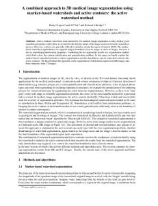
For reducing the computation time, we reduced the image resolution for the IFT algorithm 8. The original data set with a resolution in x- and y- direction of 512x512 voxel is mapped onto 64x64 voxel. This corresponds to a reduction of the image resolution by the factor 8. In z-direction the image resolution is smaller for the medical standard image processes (CT, MRT). For our CT data set the slice thickness was 2.5 mm in contrast to the pixel spacing of 0.74 mm x 0.74 mm so that the image resolution varies by the factor 4. Thus, the image resolution in z-direction was reduced only by the factor 2 to obtain the same relationships in all three directions. The 3-D data set with the reduced image resolution is called I. Furthermore an adjacent relation ρ in ℜ3 is defined by considering all pairs of voxel (p,q) ∈ I satisfying d(p,q) = 1, where d is the Euclidean distance between p und q. In the first step of the algorithm the user marks initial foreground and background regions by drawing lines interactively in few slices of this data set I. The interaction can occur alternatively on three section planes, which are parallel to the three coordinate axes (see Figure 1 at the top). In our tests less than 10 lines were sufficient for the extraction of the area of interest. The marked lines are used for the definition of the initial path costs in the data set I, which is described by a weighted and non-oriented graph G during the region-oriented segmentation, based on the IFT. Each voxel in the data set is a node of the graph, and each pair (p,q) of ρ-adjacent voxel defines a non-oriented edge in G. For our computation we use the local neighborhood ρ = six voxel. The edge costs C(p,q) are defined as the absolute difference of the gray values of the adjacent voxel according to the equation 1. C ( p, q ) = I ( p ) − I (q )
(1)
The neighborhood ρ and the costs C are used by IFT to reduce the region growing segmentation problem to an equivalent shortest-path forest problem. The initial path costs PFI for all manually marked voxels are the maximum costs from its incident edges for the defined neighborhood
PFI = max (C ( p, qi ))
(2)
i =1,.., 6
where qi is a voxel in the direct neighborhood of p. For all other voxel the initial path costs are infinite. Nodes are split into foreground and background according to the path costs. The optimal splitting of the data set is computed with dynamic programming. We use the following version of the algorithm according to 8: 1) Set PF(p) to ∞, set a label image lb(p) with the current label of each voxel to 0 for all voxel p∈I. 2) Set PF(r) to PFI(r) according equation 2 and lb(r) to its corresponding label for all marked voxel r 3) Put all voxel r in a priority queue Q 4) While Q is not empty do a) b)
Remove the voxel p with the minimal PF(p) from Q and put p in a list L of voxel which have already been processed for each ρ-adjacent voxel q of p and q∉L do (i) compute the new path cost tmp based on PF(p) and C(p,q) (ii) if tmp < PF(q) then a) set PF(q) = tmp b) set lb(q) = lb(p) c)
set the pointer with the current parents of q to p if q∉Q then insert q in Q else update position of q in Q
After this first splitting of the image the user can introduce additional start regions as model information to improve the previous result. Outgoing from these new start regions a reorganization and re-classification of the regions starts until no node can be reached at lower cost by another path. The resulting binary image is then extended to its original resolution (see Figure 1 in the middle).
2.2.
Final segmentation
The boundary between foreground and background voxel is smoothed with a boxcar filter. Subsequently, two threshold values T1 > 0.5 and T2< 0.5 are determined. It defines a search corridor for the active surface model. It consists of all voxel p with T2 ≤ p ≤ T1. The initial position of the active surface may be either the internal boundary at T=T1, the external boundary at T=T2 or the middle boundary at T = 0.5. For the example of the liver segmentation in 3-D CT images the derived search corridor from the coarse segmentation is illustrated in Figure 1 below. In the next step vertex points are determined for the initial location of the active surface (internal, external or middle boundary) by applying the marching cube algorithm 9. The number of the vertex points can be selected by the user. A small number of vertex points guarantee shorter computation time and a larger number of surface points guarantee a higher precision by the adaptation of the contour to the real contour. The surface υ is parametrically defined as
υ ( s, r ) = ( x( s, r ), y ( s, r ), z ( s, r ))
(3)
with x(s,r), y(s,r), and z(s,r) being the x, y, z co-ordinates on the surface and s, r ∈[0, 1]. The energy function to be minimized can be defined by 1 1
E (υ ) = ∫ ∫ w10 0 0
∂υ ∂υ ∂ 2υ ∂ 2υ ∂ 2υ + w01 + 2 w11 + w20 2 + w01 2 + P (v ( s, r )) dsdr ∂s ∂r ∂s∂r ∂s ∂r 2
2
2
2
2
(4)
where P is the potential associated with the external forces. The external forces cause the surface to be attracted to the real surface points of the object. They are dependent on the 3-D gradients in the image. The internal forces emanate from the shape of the surface. Their influence on the energy function depends on the selection of the coefficient wij. The coefficients w10 and w01 describe the elasticity of the shape of the surface. The rigidity of the surface is determined by w20 and w02. The parameter w11 characterized the resistance to twist. In our program the user has the choice to select the different values for these parameters. With the optimal parameter selection he/she can constrain the surface structure by adjusting boundary conditions.
2.3.
Defining of the external forces
The power of the external forces is dependent on the gradient in the image at the location of the vertex points. These external forces should move the surface to positions where the real surface is located. Although it is often assumed that surfaces are to be found at locations with the highest gray level gradient, this is not true in CT images. Here, objects to be segmented may often have a smaller gradient value than other structures in the neighborhood, such as bone or air in the intestines. Therefore, we estimate an expected gradient range gradE from the result of the coarse segmentation. Then, we use these values for the normalization and computation of external forces according to the equation 5.
P(v( s, r )) = grad E ( I ( x E , y E , z E )) − grad ( I ( x, y, z ))
(5)
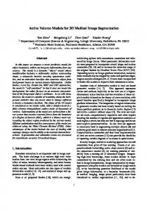
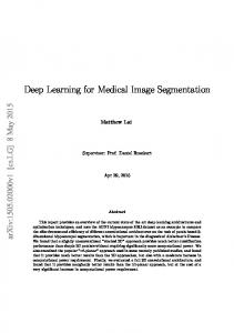
In the first step we search corresponding vertex points between the internal and external surfaces of the result of the coarse segmentation. These corresponding points are in 3-d space connected with a line. Along these lines the gray values are selected and the gray value gradients are computed. In these gradient profiles we search for the two gradient maxima between the internal boundary and the middle boundary as well as between the middle boundary and the external boundary. Off these two maxima the one is selected as ideal gradient length for external force computation, which is located closer to the middle boundary. This procedure was chosen because it is supposed that the user has the coarse segmentation carried out in this way that the middle boundary is near to the real boundary of the searched structure. Our method is illustrated in Figure 3 and Figure 4 for the example line of Figure 2. The positions for the used estimated gradient values are shown in Figure 5. In this figure you can see that the most estimated gradient values are in the correct position on the boundary of the kidney. That way the computed external forces achieve an adaptation of the active surface to the real object boundary.
Figure 2: Part of the CT image with the kidney and internal, middle and external vertex points, which are located in the slice. The line between the two corresponding points, which are located, in this case in the same slice is marked black.
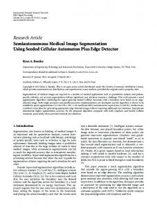
Figure 3: Profile of the gray values for the marked line in Figure 2 in direction from the internal vertex point to the external vertex point. The line shows the position of the middle boundary.
Figure 4: Gradient profile along the marked line from Figure 2. The line shows again the position of the middle boundary. The marked gradient value was selected for the gradient estimation with our algorithm.
Figure 5: Position for the estimated gradient values. The most estimated gradient values are in the correct position on the boundary between kidney tissue and surrounding structures.
3. PERFORMANCE EVALUATION OF THE ALGORITHM For evaluation of our segmentation algorithm we have used empirical discrepancy methods 10. These methods compare results with a gold standard. We selected discrepancy methods because they allow an objective and quantitative assessment of the segmentation algorithm with a close relationship to a concrete application. In our case we have used the results of the manual segmentation as the gold standard. For the tests we have had two manual segmentation results from different physicians for the three example data sets. So, we could measure a value for the intra-individual variability in the specification of the ground truth. In addition, we have had two results of the manual segmentation from one physician received on two different days for several slices of one data set. This delivered us a value for the intra-individual error.
Because the physician is interested on the volume of the segmented liver, we have used the value for the liver volume as error metric for assessment of the quality of the segmentation results. This metric has the advantage that it is independent of the region characteristics and of the segmentation method. In order to be independently of the user marking of the foreground and background regions all tests were carried out using three different coarse segmentation results.
4. RESULTS We have tested the described segmentation method for segmentation of the liver in CT data sets. The liver region exhibited only little PVE. The signal-to-noise-relation between liver tissue and surrounding structures is small. For our test data sets it was estimated to be 1:1.75. The required segmentation time was about three minutes for a data set of 512x512x90 voxel. About one minute of this time is necessary for the manual marking of the start regions and for the coarse segmentation step. The step of the active surface adaptation required about two minutes. In contrast to our two-step segmentation method the manual segmentation time of such data set was one hour. The average error for the volume determination compared with a manual segmentation that was carried out by a practicing surgeon was 8 percent. The main problem was the segmentation in the first and in the last slices. In these parts the segmented region was mostly too small because of the choice of the parameters for the internal force computation. The intra individual error for the volume determination on 25 by chance selected slices of two segmentations of one physician was 10 percent. A comparison between the inter individual error was 10 percent too. So our result was in the same range like the intra and inter individual variation. An example for the liver segmentation with our two level segmentation method is seen in Figure 6. In Figure 7 the result of this example is shown as a 3D visualization.
Figure 6: Part of a slice of the CT data set with the liver region, left: result of the manual segmentation, right: result with our two-level segmentation approach
Figure 7: 3D visualization of the result of the liver segmentation
5. DISCUSSION Parametric deformable models have been applied for many different segmentation tasks. But, they have a limitation if the designed object boundary differ greatly in size and shape from the object boundary. In our approach, we avoid this problem using user interaction. In contrast to the other segmentation approaches with parametric deformable models we need only little user interaction for defining the search corridor. Because we work in the coarse segmentation step on an image with reduced image resolution the user marking has only an insignificant influence on the defined search corridor. This influence is further reduced through the possibility of the additional marking of object and background regions until the result of the coarse segmentation is satisfactory. By an optimal choice of the search corridor, we can guarantee that the surface is located near by the real boundary after the coarse segmentation. So, the shape of the initial surface is adapted on the real object shape too. This has the advantage that the structures are founded in a short time. According to the user marking of the object we can process different topological shape with our approach.
6. CONCLUSION In this paper we presented a new process of automatically segmentation based on a two level process. In the first step of the coarse segmentation we have extracted a initial surface and a search corridor using the region based segmentation approach based on the IFT algorithm. In the second step the initial surface was adapted on the real object surface using the active surface segmentation method. We tested the practicability of this segmentation process for segmentation of liver parenchyma in CT data sets. The results of our method were compared with a manual segmentation. We found our method to work reliable. The deviation of the measured volume value between our segmentation results and manual segmentation was in the same range like the deviation between two different manual segmentations results. The deviation resulted from the different decisions about the object affiliation in the first and last slices in which the object is included. In future work we will test our approach for other medical structures and for other medical image modalities.
7. REFERENCES 1. 2. 3. 4.
5.
K.H. Höhne, W.A. Hanson, “Interactive 3D segmentation of MRI and CT volumes using morphological operations”, J. Comp. Assisted Tomogr, 16 (2), pp. 285-294, 1992. I. Cohen, L.D. Cohen, N. Ayache, “Using deformable Surfaces to segment 3-D images and infer differential structures”, CVGIP: Image Understanding, 56 (2), pp. 242-263, 1992. T.F. Cootes, C.J. Taylo, “Statistical models of appearance for medical image analysis and computer vision”, Medical Imaging 2001: Image Processing, Proc. SPIE, Vol. 4322, pp. 236-248, 2001. A. Schenk, G. Prause, H.O. Peitgen, “Efficient Semiautomatic Segmentation of 3D Objects in Medical Images“, Proc. of Medical Image Computing and Computer-assisted Intervention (MICCAI), Springer, LNCS, Vol. 1935, pp. 186-195, 2000. R. Pohle, K.D. Toennies, “Self-learning model-based segmentation of medical images”, Image Processing & Communications, 7(3-4), pp. 97-113, 2001.
6.
T. Schindewolf, H.O. Peitgen, „Interaktive Bildsegmentierung von CT- und MR-Daten auf Basis einer modifizierten Wasserscheidentransformation“, Bildverarbeitung für die Medizin, Springer, Series Informatik Aktuell, pp. 96-100, 2000. 7. V. Pekar, M.R. Kraus, C. Lorenz et. al., “Shape model based adaption of 3-D deformable meshes for segmentation of medical images”, Medical Imaging 2001: Image Processing, Proc. SPIE, Vol. 4322, pp. 281-289, 2001. 8. A.X. Falcao, R. de A. Lotufo, G. Araujo, “The Image Foresting Transformation”, Relatorio Tecnico IC-00-12, 2000. 9. C. Lorenson: Marching Cubes, “A High Resolution 3D Surface Construction Algorithm”, Computer Graphics 21, pp. 163-169, 1987. 10. Zhang Y J, “A Survey on Evaluation Methods for Image Segmentation”, Pattern Recognition, 29(8), pp. 13351346, 1996.
Figure 1: At the top: selected region of the CT image of the abdomen with marks for the liver region and marks for the background region, in the middle: result of the coarse segmentation of the liver, below: extracted search corridor for the final segmentation