rithm for the segmentation of planar regions out of 3D range · maps of urban ... to segment planar surfaces from noisy 3D range data. A pair ..... Mag., 13(3):108–.
4th European Conference on Mobile Robots – ECMR’09, September 23–25, 2009, Mlini/Dubrovnik, Croatia
Graph-based Segmentation of Range Data with Applications to 3D Urban Mapping Agustin Ortega, Ismael Haddad and Juan Andrade-Cetto Institut de Rob`otica i Inform`atica Industrial, CSIC-UPC, Barcelona, Spain
Abstract— This paper presents an efficient graph-based algorithm for the segmentation of planar regions out of 3D range maps of urban areas. Segmentation of planar surfaces in urban scenarios is challenging because the data acquired is typically sparsely sampled, incomplete, and noisy. The algorithm is motivated by Felzenszwalb’s algorithm to 2D image segmentation [8], and is extended to deal with non-uniformly sampled 3D range data using an approximate nearest neighbor search. Interpoint distances are sorted in increasing order and this list of distances is traversed growing planar regions that satisfy both local and global variation of distance and curvature. The algorithm runs in O(n log n) and compares favorably with other region growing mechanisms based on Expectation Maximization. Experiments carried out with real data acquired in an outdoor urban environment demonstrate that our approach is well-suited to segment planar surfaces from noisy 3D range data. A pair of applications of the segmented results are shown, a) to derive traversability maps, and b) to calibrate a camera network.
(a) Unsegmented map (top view)
Index Terms— 3D Segmentation, Urban Robot Mapping, Plane Extraction, Camera Network Calibration.
I. I NTRODUCTION Mobile service robots are increasingly being used for urban tasks such as guidance or search and rescue [14]. The 3D models these robots build must allow not only navigation, but should also help in path and task planning [18], or even camera network calibration [12]. Hence, these models should not only be accurate, but also tractable. Accuracy of these models is accounted for by state of the art simultaneous localization and mapping, a mature field in its own right [15, 10, 6, 7, 3, 11]. Tractability on the other hand is possible by extracting higher order primitives from the extremely large point sets these mapping algorithms produce and, relying on these primitives, to pursue higher level tasks. We present in this paper a technique to segment planar surfaces out of 3D maps of outdoor urban areas. The segmented planes can then be used to produce traversability maps, to aid in the calibration of a camera network, or to generate VR models of the scene. The proposed algorithm is very efficient since its computational complexity is O(n log n) on the number of points in the map. The method is motivated by a graph-based image segmentation algorithm [8], that has been modified to deal with non-uniformly distributed 3D range data. This work is associated with the European Project URUS (Ubiquitous Networked Robotics in Urban Settings), that puts together camera networks and mobile robots in urban pedestrian areas for people assistance tasks. Figure 1 shows an aerial view of a section of our application scenario, the Barcelona
(b) Segmented planes Fig. 1. Partial view of the Barcelona Robot Lab. The segmentation results shown correspond to a search for 30 nearest neighbors per point, 0.5 m distance threshold, and 0.5 curvature threshold.
Robot Lab, together with a plot of the segmented planes extracted with our algorithm. This map was produced with the method reported by Valencia et al., [17]. The segmentation algorithm we present is capable of segmenting maps with over 8 million points and with accuracies that range from 5 to 20 cm, and is very flexible with only three parameters to tune: a nearest-neighbor bound, and thresholds for maximum distance between points and maximum curvature for a region. The paper is organized as follows. First, an overview of related work in 3D segmentation is presented. Then, the proposed method is described in detail and compared with a 193
4th European Conference on Mobile Robots – ECMR’09, September 23–25, 2009, Mlini/Dubrovnik, Croatia
state of the art approach that uses Expectation Maximization (EM) to fit a probabilistic model of flat surfaces to the range data acquired with a mobile robot [9]. The comparison takes into account both quality of results and execution time. Finally experiments on simulated and real data are presented, followed by some concluding remarks. II. R ELATED W ORK The segmentation of 3D range maps into planar surfaces is usually addressed by region growing algorithms. The system presented by Poppinga et al., [13] for instance, contains a number of heuristics to obtain incremental plane fitting with the assumption that nearest neighbors are taken directly from the indexes in the range image. Moreover, its secondary polygonalization step is viewpoint dependent, relying also on the neighboring associations given by the indexes of the range data. In contrast, in our method, nearest neighbors are obtained using an efficient approximate nearest neighbor search over the entire 3d point map. If the number of planes to detect is known a priori, EM can be used to assign points to planes in terms of normal similarity, density of points and curvature [9]. The technique is shown for indoor scenes in which planar patches are usually orthogonal to each other. For larger, sparser point distributions, such as the ones found in outdoor range data, the assumption of a priori knowledge of the number of planes is unrealistic. To this end, hierarchical EM can be used [16], incrementally reducing the number of planes with a Bayesian information criterion, at the expense of higher computational cost. Contrary to region growing, one could search for region boundaries instead. A good exemplar of this technique is presented in an architectural modeling application [4], in which polyhedral models are generated from range data by clustering points according to their normal directions plotted on a Gaussian sphere. This mechanism helps overcome the sparsity of the point distribution. The assumption that the scene is made of planar regions is exploited to detect plane intersections and corners to compute plausible segmentations of building structures made of polyhedrons of low complexity. The method presented in this paper is motivated on a graphbased image segmentation algorithm that grows regions according to local and global region similarity in linear time [8]. Our similarity measures rely on closeness of points and normal curvature. Moreover, neighbors candidates for region growing are searched for with an Approximate Nearest Neighbor(ANN) technique [2] that runs in logarithmic time. III. G RAPH - BASED 3D S EGMENTATION Our method builds upon Felzenszwalb’s algorithm for 2D image segmentation [8], and extends it to deal with nonuniformly sampled 3D range data. The algorithm proceeds as follows. First, the entire data set is preprocessed to compute local normal orientation of fitted planar patches for each point with respect to its k-Nearest Neighbors (kNNs). Then, distances between nearest neighbors are computed. These distances are then sorted in increasing order and the resulting list is processed to create a forest of trees by merging neighboring
Fig. 2. Projections d1 and d2 of two points onto neighboring planar patches.
points according to point distances and to the angle between their normals. These two measures, the distance between neighboring points and the angle between their normals, account for local segment variation. Global segment variation is also considered by computing the angle between a point normal and the aggregated normal for the current segment, i.e., the current tree in the forest. Local and global variation are both taken into account during tree merging hypotheses. A. Fitting Normals to Local Planar Patches Consider each 3D point in the dataset with coordinates p = (x, y, z)⊤ . The error between a fitted planar patch and the range map values for the kNNs to p is given by X ǫ= (p⊤i n − d)2 , (1) i∈K
where n = (nx , ny , nz ) is the local surface normal at p, K is the set of kNNs to p, and d the distance from p to the plane. This error can be re-expressed in the following form ! ! X X ⊤ ⊤ ⊤ pi n + |K|2 d2 . ǫ=n pi pi n − 2d ⊤
|
i∈K
{z Q
}
|
i∈K
{z q
}
Combining the above error metric with the orthonormality property for each local surface normal into a Lagrangian of the form � l n⊤ , d, λ = ǫ + λ(1 − n⊤ n) , the local surface normal that best fits the patch K is the one that minimizes the above expression [1]. Deriving l with respect to n and d, and setting the derivatives to zero, it turns out that the solution is the eigenvector associated to the smallest eigenvalue of � � q qT Q − |K| n = λn . 2 B. Segmentation Criteria Once local surface normals and planar patches are computed for each point in the 3D data, segments are merged in a forest of trees based on curvature and mean distance. The curvature is defined as the angle between two normals for two matching segments, and it must be below a user-defined threshold tc , 194
4th European Conference on Mobile Robots – ECMR’09, September 23–25, 2009, Mlini/Dubrovnik, Croatia
(a) before union by rank Fig. 3.
(b) after union by rank
(c) path compression
Operations used to maintain the height of trees minimal during the merge of planar patches.
|cos−1 (n⊤1 n2 )| < tc . To account for global variation, two segments passing the curvature criteria are joined if their weighted distance is below a user selected threshold td , k1 d1 +k2 d2 k1 +k2
< td ,
the bottleneck of the algorithm is nearest neighbor search. The overall expected computational complexity of our range data segmentation algorithm is O(n log n), with worst case computational complexity O(n2 ) for ill posed distributions of the 3d points. This complexity is in contrast to the much more expensive iterative algorithms that relay on EM.
with d1 = (p1 − p2 )⊤ n2 , d2 = (p2 − p1 )⊤ n1 , where k1 and k2 are the total number of points each segment holds, and d1 and d2 , the distances between points p1 and p2 and the planes (see Fig. 2). C. Implementation Details Input parameters to the segmentation algorithm are |K| the number of local neighbors to consider for the fitting of planar patches, a distance threshold td , and a curvature threshold tc . Each planar patch is stored in a tree structure. The tree contains in each node a 3D point belonging to the segment. The parent node contains also the surface normal. The entire scene is thus represented as a forest of disjoint trees. At each iteration over the list of ordered distances, the merging of neighboring planar patches is hypothesized. If the local and global variation criteria are satisfied, both in terms of neighboring distance and curvature, the segments are joined using union by rank and path compression. Union by rank means choosing as tree root the one with larger cardinality when merging two trees, thus minimizing the depth of the tree. Path compression makes all nodes on a tree point to its parent, thus effectively reducing the tree depth to 1 [5] (see Fig. 3). D. Computational Complexity Analysis The ANN library we use to search for approximate nearest neighbors has expected computational complexity O(log n) [2], and worst case complexity O(n). Moreover, the complexity of union by rank and path compression is worst case O(α(n)) where α(n) is the very slowly growing inverse of Ackermann’s function [5], which for any conceivable application is α(n) < 4. Therefore, our region growing algorithm takes linear time in the number of points in the dataset, and
IV. E XPERIMENTS The proposed algorithm was tested using synthetic and real data. In the first experiment we built a synthetic model of an open 3D box consisting of five equally sized faces with varying noise parameters and also with various levels of outliers to account for unstructuredness in the scene. For each plane, N 2D points are drawn from a uniform distribution in 3D. Then, each point is corrupted with zero mean Gaussian noise with independent variance σ 2 on each axis. Finally, a small percentage of these points is further normally corrupted with three times variance σ 2 to simulate the presence of outliers. We used the following values in the simulation: σ 2 = {0.0001, 0.001, 0.01, 0.1, 0.2, 0.3, 0.4, 0.5}, percentage of outliers equal to 5%, 10%, and N = 1000 points per plane, i.e., 5000 points per open cube. The proposed algorithm was compared with Liu’s EM algorithm [9]. In our implementation of Liu’s method, the following parameters were used: J = 5 planes; points are considered outliers when xmax > 2; and the density of each plane is smaller than 70% of the simulated points. The terminating condition in the standard EM algorithm is reached when J = 5 planes are found and the E and M steps have iterated over 25 cycles. Figure 4 shows cubes generated with 5% and 10% of outliers and noise parameters σ 2 = 0.0001 and σ 2 = 0.001. A comparison of Liu’s method to ours is shown in Fig. 4. Figure 5 shows the mean square reprojection error for each plane ǫ/N , computed from Eq. 1, and averaged for all planes in the open cube. For the selected operating parameters, both methods have comparable segmentation results. The clear advantage of the proposed algorithm is its computational cost. To compare algorithm speed, the open cube is sampled with N = {100, 500, 1000, 5000}, a fixed 1% amount of outliers, variance σ 2 = 0.01, and maximum iteration to 25 cycles for the EM algorithm. Fig. 6 reports execution 195
4th European Conference on Mobile Robots – ECMR’09, September 23–25, 2009, Mlini/Dubrovnik, Croatia
(a) Synthetic data with σ 2 = 0.0001 and 5% of outliers
(b) EM-based segmentation results
(c) Graph-based segmentation results
(d) Synthetic data with σ 2 = 0.001 and 10% of outliers
(e) EM-based segmentation results
(f) Graph-based segmentation results
Fig. 4. Synthetically generated data for an open cube with five faces. Expectation-maximization-based segmentation is computed with our implementation of the method reported in [9]. The last column shows segmentation results over the same data with the proposed graph-based segmentation algorithm.
5% percent of outliers
10% percent of outliers 1
Liu Our Method
0.9
0.9
0.8
0.8 Mean Square Error
Mean Square Error
1
0.7
0.6
0.7
0.6
0.5
0.5
0.4
0.4
0
0.1
0.2
0.3
0.4
Liu Our Method
0.5
0
0.1
0.2
Variance
(a) Reprojection error with 5% of outliers Fig. 5.
0.3
0.4
0.5
Variance
(b) Reprojection error with 10% of outliers
Mean square reprojection error with varying noise parameters and percentage of outliers for the two segmentation algorithms.
Time Vs Points
Time Vs Points
450
3.5 Our Method
Liu Our Method
400
3
350 300
Time in Seconds
Time in Seconds
2.5
250 200
2
1.5
150 1 100 0.5
50 0
0
1000
2000 3000 Number Points
4000
(a) Execution time for both algorithms Fig. 6.
0
5000
0
1000
2000 3000 Number Points
4000
5000
(b) Execution time for the proposed approach
Time comparison between EM-based segmentation and the proposed graph-based approach.
196
4th European Conference on Mobile Robots – ECMR’09, September 23–25, 2009, Mlini/Dubrovnik, Croatia
(a) Planes extracted from the map of the Barcelona Robot Lab with the proposed graph-based segmentation approach
Fig. 7.
Aerial view of the Barcelona Robot Lab, and its 3D point map.
times for both the EM-based and our graph-based segmentation approaches. In spite that the expected computational complexity of our algorithm is O(n log n), its constant factor is significantly smaller than that of the EM-method. At 5000 data points, our method takes only about 3 seconds, whereas the EM-based approach is over 150 times slower, taking more than 7 minutes to compute the segmentation, in our implementation. All reported times are for experiments performed in a Pentium 4 PC with 2GB RAM running Matlab under Linux. The method is applied to our real data set of the Barcelona Robot Lab, acquired during an outdoor 3D laser-based SLAM session [17]. The set contains over 8 million points and maps the environment with accuracies that vary from 5 cm to 20 cm approximately. The input parameters for our segmentation algorithm applied to this set are K = 30 nearest neighbors, td = 0.5 for distance threshold, and tc = 0.5 for curvature threshold. Segmentation results are shown in Fig. 8. The proposed algorithm takes approximately 20 minutes to complete the plane segmentation. To show the applicability of the algorithm to robotics tasks, segments are labeled according to their normal orientation to indicate traversable regions versus walls and obstacles. Another example of the use of our segmentation method is camera network calibration. In this case, the segmented planes are further intersected to find lines which correspond to architectural features on the scene. Lines lying orthogonally, i.e., with orientations within ±0.03 of 0 and pi 2 along the three axes, were further projected onto camera images and matched with image features. Feature matching is refined through a minimization process over both extrinsic and intrinsic camera parameters as detailed in [12]. The result is a camera calibration for the entire camera network. Figure 9 shows the segmented data set reprojected onto the image on one of the cameras, line feature matches, and the results of the calibration routine in the form of a computed homography to the ground plane.
(b) A possible application of the algorithm is to label segments according to traversability conditions Fig. 8. Barcelona Robot Lab. The segmentation results help differentiate horizontal planes for traversability (in red) from walls and obstacles (in blue).
V. C ONCLUSIONS AND F UTURE W ORK The presented technique to range data segmentation into planar segments has several advantages when compared to region merging EM-based algorithms. On the one hand, the computational cost of the presented approach is very appealing to large point clouds. Moreover, no a priori knowledge on the number of planes in the scene is needed. Experiments carried out with real datasets acquired in an outdoor urban environment demonstrate its applicability to various robotics applications, including the computation of traversability maps and camera network calibration. Further refinements to our approach include the extraction of texture from the calibrated images and some polygonalization strategy with the aim of producing realistic VR models of large scenes.
ACKNOWLEDGMENT This work has been partially supported by the Mexican Council of Science and Technology under a PhD Scholarship to Agustin Ortega, by the Spanish Ministry of Science and Innovation under projects DPI-2008-06022 and MIPRCV Consolider-Ingenio 2010, and by the EU URUS project ISTFP6-STREP-045062. The authors thank M. Morta for the development of the 3D scanner used for this work. 197
4th European Conference on Mobile Robots – ECMR’09, September 23–25, 2009, Mlini/Dubrovnik, Croatia
R EFERENCES [1] J. Andrade-Cetto and A. C. Kak. Object recognition. In J. G. Webster, editor, Wiley Encyclopedia of Electrical and Electronics Engineering, supplement 1, pages 449–470. John Wiley & Sons, New York, 2000. [2] S. Arya, D. M. Mount, N. S. Netanyahu, R. Silverman, and A. Y. Wu. An optimal algorithm for approximate nearest neighbor searching fixed dimensions. J. ACM, 45(6):891–923, Nov. 1998. [3] T. Bailey and H. Durrant-Whyte. Simultaneous localisation and mapping (SLAM): Part II state of the art. IEEE Robot. Automat. Mag., 13(3):108– 117, Sep. 2006. [4] J. Chen and B. Chen. Architectural modeling from sparsely scanned range data. Int. J. Comput. Vision, 78(2-3), 2008. [5] T. H. Cormen, C. E. Leiserson, and R. L. Rivest. Introduction to Algorithms. MIT Electrical Engineering and Computer Science Series. MIT Press, Cambridge, 1992. [6] F. Dellaert and M. Kaess. Square root SAM: Simultaneous localization and mapping via square root information smoothing. Int. J. Robot. Res., 25(12):1181–1204, 2006. [7] R. M. Eustice, H. Singh, and J. J. Leonard. Exactly sparse delayed-state filters for view-based SLAM. IEEE Trans. Robot., 22(6):1100–1114, Dec. 2006. [8] P. F. Felzenszwalb and D. P. Huttenlocher. Efficient graph-based image segmentation. Int. J. Comput. Vision, 59(2):167–181, Sep. 2004. [9] Y. Liu, R. Emery, D. Chakrabarti, W. Burgard, and S. Thrun. Using EM to learn 3D models of indoor environments with mobile robots. In Proc. 18th Int. Conf. Machine Learning, pages 329–336, Williamstown, Jul. 2001. [10] M. Montemerlo and S. Thrun. FastSLAM: A Scalable Method for the Simultaneous Localization and Mapping Problem in Robotics, volume 27 of Springer Tracts in Advanced Robotics. Springer, 2007. [11] A. N¨uchter, K. Lingemann, J. Hertzberg, and H. Surmann. 6D SLAM3D mapping outdoor environments. J. Field Robot., 24(8-9):699–722, 2007. [12] A. Ortega, B. Dias, E. Teniente, A. Bernardino, J. Gaspar, and Juan Andrade-Cetto. Calibrating an outdoor distributed camera network using laser range finder data. In Proc. IEEE/RSJ Int. Conf. Intell. Robots Syst., Saint Louis, Oct. 2009. To appear. [13] J. Poppinga, N. Vaskevicius, A. Birk, and K. Pathak. Fast plane detection and polygonalization in noisy 3D range images. In Proc. IEEE/RSJ Int. Conf. Intell. Robots Syst., pages 3378–3383, Nice, Sep. 2008. [14] A. Sanfeliu and J. Andrade-Cetto. Ubiquitous networking robotics in urban settings. In Proc. IEEE/RSJ IROS Workshop Network Robot Syst., pages 14–18, Beijing, Oct. 2006. [15] S. Thrun, W. Burgard, and D. Fox. Probabilistic Robotics. MIT Press, Cambridge, 2005. [16] R. Triebel, W. Burgard, and F. Dellaert. Using hierarchical EM to extract planes from 3D range scans. In Proc. IEEE Int. Conf. Robot. Automat., pages 4437–4442, Barcelona, Apr. 2005. [17] R. Valencia, E.H. Teniente, E. Trulls, and J. Andrade-Cetto. 3D mapping for urban serviece robots. In Proc. IEEE/RSJ Int. Conf. Intell. Robots Syst., Saint Louis, Oct. 2009. To appear. [18] O. Wulf, C. Brenneke, and B. Wagner. Colored 2D maps for robot navigation with 3D sensor data. In Proc. IEEE/RSJ Int. Conf. Intell. Robots Syst., pages 2991–2996, Sendei, Sep. 2004.
(a) Segmented range data projected to a camera image.
(b) Plane boundaries used for camera calibration.
(c) Calibration results are used to recover an orthographic view of the scene. Fig. 9. Application of the segmentation method for the calibration of an outdoor camera network. Plane boundaries and plane intersections are projected to the image of one of the cameras in the network. A nonlinear optimization of the projection error is used to refine the calibration parameters.
198