SS symmetry Article
Segmentation of Brain Tumors in MRI Images Using Three-Dimensional Active Contour without Edge Ali M. Hasan 1,2 , Farid Meziane 1 , Rob Aspin 1 and Hamid A. Jalab 3, * 1 2 3
*
School of Computing, Science and Engineering, University of Salford, Manchester M5 4WT, UK;
[email protected] (A.M.H.);
[email protected] (F.M.);
[email protected] (R.A.) Computers Unit, College of Medicine, Al-Nahrain University, Baghdad 64074, Iraq Faculty of Computer Science & Information Technology, University of Malaya, Kuala Lumpur 50603, Malaysia Correspondence:
[email protected]; Tel.: +60-3-7967-2503
Academic Editor: Angel Garrido Received: 13 October 2016; Accepted: 14 November 2016; Published: 18 November 2016
Abstract: Brain tumor segmentation in magnetic resonance imaging (MRI) is considered a complex procedure because of the variability of tumor shapes and the complexity of determining the tumor location, size, and texture. Manual tumor segmentation is a time-consuming task highly prone to human error. Hence, this study proposes an automated method that can identify tumor slices and segment the tumor across all image slices in volumetric MRI brain scans. First, a set of algorithms in the pre-processing stage is used to clean and standardize the collected data. A modified gray-level co-occurrence matrix and Analysis of Variance (ANOVA) are employed for feature extraction and feature selection, respectively. A multi-layer perceptron neural network is adopted as a classifier, and a bounding 3D-box-based genetic algorithm is used to identify the location of pathological tissues in the MRI slices. Finally, the 3D active contour without edge is applied to segment the brain tumors in volumetric MRI scans. The experimental dataset consists of 165 patient images collected from the MRI Unit of Al-Kadhimiya Teaching Hospital in Iraq. Results of the tumor segmentation achieved an accuracy of 89% ± 4.7% compared with manual processes. Keywords: magnetic resonance imaging; modified gray level co-occurrence matrix; three-dimensional active contour without edge; two-dimensional active contour without edge
1. Introduction Brain tumors are relatively less common than other neoplasms, such as those of the lung and breast, but are considered highly important because of prognostic effects and high morbidity [1]. Clinical diagnosis, predicted prognosis, and treatment are significantly affected by the accurate detection and segmentation of brain tumors and stroke lesions [2]. The Iraqi Ministry of Health reported that the use of depleted uranium and other toxic substances in the first and second Gulf Wars had increased the average annual number of registered cancerous brain tumor cases and birth defects since 1990 [3]. This study was conducted in collaboration with MRI units in Iraqi hospitals that have witnessed the high numbers of these cases. The role of image processing in medicine has expanded with the progress of medical imaging technologies, and additional images are obtained using an increased number of acquisition modalities. Therefore, image processing was embedded in medical systems and used widely in medicine, from diagnosis to therapy. To date, diagnostic imaging is an invaluable tool in medicine. Standard medical imaging techniques, such as ultrasonography, computed tomography, and magnetic resonance imaging (MRI), have significantly increased knowledge on anatomy and disease diagnosis in medical research. Among these medical technologies, MRI is considered a more useful and appropriate imaging technique for brain Symmetry 2016, 8, 132; doi:10.3390/sym8110132
www.mdpi.com/journal/symmetry
Symmetry 2016, 8, 132
2 of 21
tumors than other modalities. MRI presents detailed information on the type, position, and size of tumors in a noninvasive manner. Additionally, MRI is more sensitive to local changes in tissue density. Spatial resolution, which represents the digitization process of assigning a number to each pixel in the original image, has increased significantly in recent years. Standard MRI protocols are commonly used to produce multiple images of the same tissue with different contrast after the administration of parametric agents, including T1-weighted (T1-w), T2-weighted (T2-w), fluid-attenuated inversion recovery (FLAIR), and T1-weighted images with contrast enhancement (T1c-w). T1-w images are obtained during the T1 relaxation time of the excited net magnetization or protons to recover 63% of the original net magnetization after the radiofrequency pulse of the MRI scanner is switched off. By contrast, T2-w images are obtained during T2 relaxation time, which represents the required time for the decline of net magnetization to 37% of the original net magnetization [4]. FLAIR is a special protocol in MRI scanners and produces adaptive T2-w images by removing the signal of brain edema and other structures with high water content, such as cerebrospinal fluid (CSF) [5]. Most brain tumors appear as hypo-intense relative to normal brain tissue on T1-w images and hyper-intense on T2-w images. Therefore, T2-w images are commonly used for providing an initial assessment, identifying tumor types, and distinguishing tumors from non-tumor tissues [6]. A contrast material is commonly used to enhance the tumor boundary against the surrounding normal brain tissue on T1-w images. This technique enables tumor detection that cannot be distinguished and recognized from T2-w and T1-w images because of similarity with adjacent normal brain tissue [7]. In clinical routine, a T2-w scan is performed immediately after patient positioning to identify the tumor location. T1-w scan is used before and after contrast administration for tumors showing contrast enhancement. The T2-w scan in axial viewing with FLAIR is used to show non-enhanced tumors [6]. As scanner resolutions improved and slice thickness decreased, an increasing number of slices were produced and clinicians required increasing time to diagnose each patient from image sets. Therefore, automated tumor detection and segmentation have attracted considerable attention in the past two decades [8]. One particular challenge in imaging features is the similarity between tumors located inside the brain white matter and those that overlap intensity distributions with the gray matter. This pattern is particularly evident at the boundary between a tumor and the surrounding tissue. Partial volumes (PVs) are considered as boundary features containing a mixture of different tissue types [9]. The thicknesses of the image slices (5–7 mm) produce significant PV effects, in which individual image pixels describe more than one tissue type. As a result, peripheral tumor regions are misclassified. This occurrence is common in T2-w images. A similar problem occurs toward the outer brain edge, where the CSF and gray matter overlap with the image sample. This circumstance may generate image intensities that erroneously indicate tumor presence. In the past few decades, the number of studies devoted to automated brain tumor segmentation has grown rapidly because of the progress in the medical imaging field [8]. Active contour models, or snakes, are highly important applications for brain tumor segmentation. These tools are strongly suitable for determining the boundary between the tumor and the surrounding tissue [10]. This approach enables segmentation, matching, and tracking of anatomical areas by exploiting conditions derived from the anatomical and biological knowledge regarding location, size, and shape of anatomical areas [11]. Active contour models are defined as curves or surfaces that move under the influence of weighted internal and external forces. Internal forces are responsible for curve smoothness, whereas external forces are responsible for the pushing and pulling of curves toward the anatomical area boundaries. Generally, the active contour models suffer from the problem of initial contour determination and leakage in imprecise edges. The majority of the proposed approaches in brain abnormality detection and segmentation are limited by (i) computational complexity; the (ii) absence of full automation because of brain tumor diversity; and (iii) the problem of contour initialization and imprecise edges.
Symmetry 2016, 8, 132
3 of 21
To overcome these problems, we developed a fully automated method for locating the initial contour and segmentation of brain tumors by using a three-dimensional active contour without edge (3DACWE). Moreover, we compared the resulting accuracies of 2D and 3D segmentations. Our system is based on the use of a single MRI modality (T2-w images) in axial viewing for detecting brain abnormality instead of multi-modal MRI (e.g., sagittal and coronal images). The system searches in parallel for dissimilar regions corresponding to its reflection on the opposite hemisphere of the brain by exploiting normal brain structural symmetry. This method would help commence the segmentation process automatically. Consequently, the proposed system becomes fully automated and is independent from atlas registration to avoid any inaccurate registration process that may directly affect the precision of tumor segmentation. Such a strategy also does not require a prior skull-removing step. The remaining sections of this paper are organized as follows: in Section 2, the proposed method is explained; in Section 3, experimental results are discussed while describing how to locate and identify the tumor; and in Section 3, the conclusions are given. 2. Proposed Method This research aimed to develop an automated method that can locate the initial contour of brain tumor segmentation across all axial slices of volumetric MRI brain scans. The overall flow chart of the proposed method is shown in Figure 1. 2.1. Data Collection The clinical image dataset consists of 165 MRI brain scans acquired during routine diagnostic procedure at the MRI Unit in Al-Kadhimiya Teaching Hospital in Baghdad, Iraq. This dataset was diagnosed and classified into normal and abnormal by the clinicians of this unit. The MRI slice sets were obtained using a SIEMENS MAGNETOM Avanto 1.5 Tesla scanner (Malvern, PA, USA) and PHILIPS Achieva 1.5 Tesla scanner (Best, Netherlands). The provided dataset consisted of tumors with different sizes, shapes, locations, orientations, and types. A total of 88 patients in this dataset exhibited different brain abnormalities with tumor sizes, shapes, locations, orientations, and types. The remaining patient images exhibited no detectable pathology. The dataset included the four MRI image modalities, namely, T2-w, T1-w, T1c-w, and FLAIR images, under axial viewing and 3–5 mm slice thickness. An additional enhanced dataset of 50 pathological patients was prepared, although the brain tumors were manually segmented and labeled by an expert in this unit who evaluates segmentation algorithm accuracy. The standard benchmark Multimodal Brain Tumor Segmentation dataset (BRATS 2013) obtained from the International Conference on Medical Image Computing and Computer-Assisted Interventions [8] was adopted to evaluate the proposed method. 2.2. Image Preprocessing The preprocessing step involved the performance of a set of algorithms on MRI brain scan slices as a preparation for the feature extraction step. This step included dimension resizing of the MRI slices, image enhancement by Gaussian filter, and normalization of MRI image intensity because of image intensity variation. Finally, mid-sagittal plane (MSP) detection and correction algorithm were implemented.
Symmetry 2016, 8, 132 Symmetry 2016, 8, 132
4 of 21 4 of 21
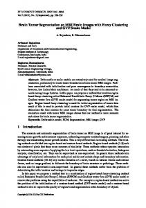
Figure 1. Flowchart of the proposed algorithm. Figure 1. Flowchart of the proposed algorithm.
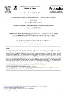
2.2.1. Resizing the Dimensions of MRI (Magnetic Resonance Imaging) Slices 2.2.1. Resizing the Dimensions of MRI (Magnetic Resonance Imaging) Slices The provided MRI MRI brain slices collected from two scanners with spatial different spatial The provided brain slices werewere collected from two scanners with different resolutions. resolutions. To enable the use of the full set without bias, the MRI scans were resized to 512 × 512 To enable the use of the full set without bias, the MRI scans were resized to 512 × 512 pixels. pixels. All algorithms developed in this were implemented on squared slices. When the All algorithms developed in this study werestudy implemented on squared slices. When the dimensions of dimensions of the given MRI slices were changed to a square ratio, care was taken to maintain the the given MRI slices were changed to a square ratio, care was taken to maintain the ratio of voxels to ratio of voxels to pixels (e.g., pixel spacing). The MRI slices were then resized by adding additional pixels (e.g., pixel spacing). The MRI slices were then resized by adding additional columns from the columns from the left and right and additional rows from the top and bottom portions of the MRI left and right and additional rows from the top and bottom portions of the MRI slice until the slice size slice until the slice size became 512 × 512 pixels in resolution (Figure 2). became 512 × 512 pixels in resolution (Figure 2).
Symmetry 2016, 8, 132
5 of 21
Symmetry 2016, 8, 132
5 of 21
Figure 2. Padding of MRI brain image margins by zeros.
Figure 2. Padding of MRI brain image margins by zeros. 2.2.2. MRI Enhancement Algorithm
2.2.2. MRI Enhancement Algorithm
The typical noise in MRI images appeared as a small random modification of the intensity in an individual or a small groups of pixels. These differences can be sufficiently large to lead to erroneous The typical noise in MRI images appeared as a small random modification of the intensity segmentation. A spatial domain low‐pass filter (Gaussian filter, The Math Works, Natick, MA, USA) in an individual or a small groups of pixels. These differences can be sufficiently large to lead to was used and contributed a negative effect to the responses of noise smoothing linear image erroneous segmentation. A spatial domain low-pass filter (Gaussian filter, The Math Works, Natick, enhancement. Consequently, the performance of the Gaussian filter was evaluated visually because MA, USA) was used and contributed a negative effect to the responses of noise smoothing linear image of its preferably low value for σ [11,12].
enhancement. Consequently, the performance of the Gaussian filter was evaluated visually because of 2.2.3. Intensity Normalization its preferably low value for σ [11,12]. The pixel intensity values of each MRI slice were normalized to the same intensity interval to
2.2.3. Intensity Normalization achieve dynamic range consistency. Histogram normalization was then applied to stretch and shift the original histogram of the image and cover all the grayscale levels in the image. The resulting
The pixel intensity values of each MRI slice were normalized to the same intensity interval normalized image achieved a higher contrast than that of the original image because the histogram to achieve dynamic method range consistency. Histogram normalization was then to stretch normalization enhanced image contrast and provided a wider range applied of intensity and shift the original histogram of the image and cover all the grayscale levels in the transformation. This approach demonstrated an enhanced classification of pathological tissues that image. can be achieved using the unmodified image [13]. The resulting normalized image achieved a higher contrast than that of the original image because the histogram normalization method enhanced image contrast and provided a wider range of intensity 2.2.4. Background Segmentation transformation. This approach demonstrated an enhanced classification of pathological tissues that Prior using knowledge suggests that the background intensity values of MRI brain slices often can be achieved the unmodified image [13]. approaches zero to enable background segmentation. The ability to eliminate and exclude the background the region of interest is important because the background normally contains a 2.2.4. Background from Segmentation much higher number of pixels than that of the brain region but without meaningful information [13]. Prior knowledge suggests that the background intensity values of MRI brain slices often In this study, histogram thresholding was used as a segmentation method to isolate the background. This approach is based on the thresholding of intensity values by a specific T value. Subsequently, approaches zero to enable background segmentation. The ability to eliminate and exclude the the application employs a set of morphological operators to remove any hole appearing in the region. background from the region of interest is important because the background normally contains Notably, the T2‐w MR image histograms attained almost identical distribution shapes [14]. Therefore, a much higher number of pixels than that of the brain region but without meaningful information [13]. the T value was selected experimentally and set to 0.1 after the effects of a range of threshold values In this study, histogram thresholding was used as a segmentation method to isolate the background. (0.05, 0.1, 0.2, and 0.3) were manually observed. Hence, if an intensity value of a pixel is less than 0.1, This approach is based on the thresholding of intensity values by a specific T value. Subsequently, the pixel is considered as a background.
the application employs a set of morphological operators to remove any hole appearing in the region. Notably,2.2.5. Mid‐Sagittal Plane Detection and Correction the T2-w MR image histograms attained almost identical distribution shapes [14]. Therefore, the T value Mid‐sagittal plane identification is an important initial step in brain image analysis because this was selected experimentally and set to 0.1 after the effects of a range of threshold values method provides an initial estimation of the brain’s pathology assessment and tumor detection. The (0.05, 0.1, 0.2, and 0.3) were manually observed. Hence, if an intensity value of a pixel is less than 0.1, the pixelhuman brain is divided into two hemispheres with an approximately bilateral symmetry around the is considered as a background.
MSP. The two hemispheres are separated by the longitudinal fissure, which represents a membrane between the left and right hemisphere. MSP extraction methods can be divided into two groups as 2.2.5. Mid-Sagittal Plane Detection and Correction follows. Content‐based methods find a plane that maximizes a symmetrical measure between both sides of the brain. By contrast, shape‐based methods use the inter‐hemispheric fissure as a simple Mid-sagittal plane identification is an important initial step in brain image analysis because landmark to extract and detect the MSP. In this study, we focused on determining the orientation of this method provides an initial estimation of the brain’s pathology assessment and tumor detection. the patient’s head instead of measuring the symmetry to identify the brain MSP [3].
The human brain is divided into two hemispheres with an approximately bilateral symmetry around the MSP. The two hemispheres are separated by the longitudinal fissure, which represents a membrane between the left and right hemisphere. MSP extraction methods can be divided into two groups as follows. Content-based methods find a plane that maximizes a symmetrical measure between both sides of the brain. By contrast, shape-based methods use the inter-hemispheric fissure as a simple landmark to extract and detect the MSP. In this study, we focused on determining the orientation of the patient’s head instead of measuring the symmetry to identify the brain MSP [3].
Symmetry 2016, 8, 132
6 of 21
2.3. Feature Extraction The fundamental objective of any diagnostic medical imaging investigation is tissue characterization. Texture analysis is commonly used to provide unique information on the intensity variation of spatially related pixels in medical images [2]. The choice of an appropriate technique for feature extraction depends on the particular image and application [4]. Texture features are extracted from MRI brain slices to encode clinically valuable information by using modified gray-level co-occurrence matrix (MGLCM). This method is a second-order statistical method proposed by Hasan and Meziane [3] to generate textural features and provide information about the patterning of MRI brain scan textures. These features are used to measure statistically the degree of symmetry between the two brain hemispheres. Symmetry is an important indicator that can be used to detect the normality and abnormality of the human brain. MGLCM generates texture features by computing the spatial relationship of the joint frequencies of all pairwise combinations of gray-level configuration of each pixel in the left hemisphere. These pixels are considered as reference pixels, with one of nine opposite pixels existing in the right hemisphere under nine offsets and one distance. Therefore, nine co-occurrence matrices are generated for each MRI brain scanning image. To reduce the dimensionality of the feature space, we added the resultant MGLCM matrices of all the MRI slices at all orientations. The maximum number of gray levels considered for each image was typically scaled down to 256 gray levels (8 bits/pixel), rather than using the full dynamic range of 65,536 gray levels (16 bits/pixel) before computing the MGLCM. This quantization step was essential to reduce a large number of zero-valued entries in the co-occurrence matrix [15,16]. The computing time for implementing MGLCM for each slice was about 2.3 min by using an HP workstation Z820 (Natick, MA, USA) with Xeon E5-3.8 GHz (Quad-Core) and 16 GB of RAM (random access memory). 2.3.1. Feature Aggregation The MGLCM method determines nine co-occurrence matrices. For each matrix, 21 statistical descriptors are determined, generating 189 descriptors for each MRI brain scan [3]. The cross correlation descriptor is also determined for the original MRI brain scan. Accordingly, 190 descriptors are attained for each MRI brain scan image. These features are used by the subsequent classification to differentiate between normal and abnormal brain images. 2.3.2. Feature Selection High-dimensional feature sets can negatively affect the classification results because high numbers of features may reduce the classification accuracy owing to the redundancy or irrelevance of some features. Feature-selection techniques aim to identify a small subset of features that minimizes redundancy and maximizes relevancy. Therefore, feature selection is an important step in exposing the most informative features and for optimally tuning the classifier’s performance to reliably classify unknown data. In this study, ANOVA was employed to measure feature significance and relevance [3]. 2.4. Classification Classification is the process of sorting objects in images into separate classes and plays an important role in medical imaging, especially in tumor detection and classification. This step is also a common process employed in many other applications, such as robotic and speech recognition [4]. In the present study, a multi-layer perceptron neural network (MLP) was adopted to classify MRI brain scans into normal and abnormal images. MLP is used in different applications, such as optimization, classification, and feature extraction [3]. 2.5. Brain Tumors Location Identification Many tumor-segmentation methods are not fully automated. These approaches require user involvement in selecting a seed point. Usually, the MRI slices of a patient are interpreted visually
Symmetry 2016, 8, 132
245 246 247 248 249 250 251 252 253 254 255 256 257 258 259 260 261 262 263 264 265 266 267 268 269 270 271 272 273 274 275 276 277 278 279 280 281 282 283
7 of 21
and subjectively by radiologists, in which tumors are segmented by hand or by semi-automatic tools. Both manual and semiautomatic approaches are considered as tedious, time-consuming, error-prone processes. Tumors are more condensed than the surrounding material and present as brighter pixels than the surrounding brain tissue. Therefore, the basic concept of brain tumor detection algorithms is Symmetry x FOR PEER REVIEW of 22 finding2016, pixel8,clusters with a different or higher intensity than that of their surroundings. In this 7study, a bounding 3D-box-based genetic algorithm (BBBGA) method was proposed by Hasan [17] to search left right the hemispheres the brain automatically withoutthe theleft need user interaction.of The andand identify location ofofmost dissimilar regions between andfor right hemispheres theinput brain was a set of MR slices belonging to the scans of a single patient, and its output was a subset of slices automatically without the need for user interaction. The input was a set of MR slices belonging to the covering circumscribing tumor was withaasubset 3D box. The BBBGA method exploits the symmetry scans of aand single patient, and the its output of slices covering and circumscribing the tumor feature of axial viewing of MRI brain slices to search for the most dissimilar region theslices left with a 3D box. The BBBGA method exploits the symmetry feature of axial viewing ofbetween MRI brain and right brain hemispheres. dissimilarity is brain detected using This GA dissimilarity and an to search for the most dissimilar regionThis between the left and right hemispheres. objective-function-based mean intensity computation. The process involves randomly generating is detected using genetic algorithm (GA) and an objective-function-based mean intensity computation. hundreds of 3D boxesrandomly with different sizes and locations in the leftwith braindifferent hemisphere. Suchlocations boxes arein The process involves generating hundreds of 3D boxes sizes and then compared with the corresponding 3Dthen boxes in the right hemisphere through theinobjective the left brain hemisphere. Such boxes are compared withbrain the corresponding 3D boxes the right function. These 3D boxes are moved and updated during the iterations of the GA toward region brain hemisphere through the objective function. These 3D boxes are moved and updatedthe during the that maximized the objective function value. An advantage of the BBBGA method is its lack of iterations of the GA toward the region that maximized the objective function value. An advantage necessity for image registration or intensity standardization in MR slices. The approach is an of the BBBGA method is its lack of necessity for image registration or intensity standardization in unsupervised hence, problems method; on observer variability in supervised techniques are MR slices. Themethod; approach is an the unsupervised hence, the problems on observer variability in ignored. supervised techniques are ignored. Prior BBBGA,exponential exponentialtransformation transformation is implemented to compress the low-contrast Prior to to BBBGA, is implemented to compress the low-contrast regions regions in MRI brain images and expand the high-contrast regions in a nonlinear manner. This in MRI brain images and expand the high-contrast regions in a nonlinear manner. This action would action would increase the intensity difference between the and brainthe tumor and the surrounding soft increase the intensity difference between the brain tumor surrounding soft tissue [17,18]. tissue [10, 11]. Fig. 3 illustrates the pseudo-code for BBBGA. Figure 3 illustrates the pseudo-code for BBBGA.
1. 2. 3. 4. 5. 6. 7. 8. 9. 10. 11. 12. 13. 14. 15. 16. 17. 18. 19.
read Img MRI slices Img exp(Img) // Initialization generate N feasible individuals ind randomly in current population , which is set experimentally to 100. compute mean(Img(ind i)) for each i ∈ N // loop until termination condition is achieved for i = 1 to N // Selection select the best two individual from current population (ind 1, ind 2) // Crossover newind 1, newind 2 with crossover-probability crossover ind 1, ind 2 // Mutation newind 1 with mutation-probability mutate ind 1 newind 2 with mutation-probability mutate ind 2 // Evaluation newind 1, newind 2 compute mean(Img(newind 1)) compute mean(Img(newind 2)) new population newind1, newind2 endfor
284
Figure3.3.Pseudo-code Pseudo-codefor forBBBGA. BBBGA. Figure
285 286 287 288 289 290 291 292
For additional additional details on thethe GAGA population is mapped into into binary form, For on how howeach eachindividual individualinin population is mapped binary we use the following scenario. Suppose we have a MRI brain scan (dimensions 512 × 512 × 32 pixels) form, we use the following scenario. Suppose we have a MRI brain scan (dimensions 512 × 512 × 32 of a pathological patient, each individual in the GA in population is denoted by binaryby representation pixels) of a pathological patient, each individual the GA population is the denoted the binary representation of the coordinates of one 3D box (x1, x2, y1, y2, z1, and z2). In this case, x1 and x2 represent the height of the 3D box and are subject to the constraints 1 ≤ x1 < 512 and x1 < x2 ≤ 512. Meanwhile, y1 and y2 signify the width of the 3D box and are subject to the constraints 1 ≤ y1 < 256 and y1 < y2 ≤ 256. Finally, z1 and z2 represent the depth of the 3D box and are subject to the constraints 1 ≤ z1 < 32 and z1 < z2 ≤ 32. Herein, we assume that the maximum number of MRI slices is
Symmetry 2016, 8, 132
8 of 21
of the coordinates of one 3D box (x1 , x2 , y1 , y2 , z1 , and z2 ). In this case, x1 and x2 represent the height Symmetry 2016, 8, 132 8 of 21 of the 3D box and are subject to the constraints 1 ≤ x1 < 512 and x1 < x2 ≤ 512. Meanwhile, y1 and ≤ 256. y the width of the 3D box and are subject to the constraints 1 ≤ y1