After that a level set approach is used for the surface fitting. The point cloud is constructed by manual marking in the training set. With cubic splines a denser ...
Segmentation of Medical Images Using Three-dimensional Active Shape Models Klas Josephson, Anders Ericsson, and Johan Karlsson Centre for Mathematical Sciences Lund University, Lund, Sweden {f00kj, anderse, johank}@maths.lth.se http://www.maths.lth.se
Abstract. In this paper a fully automated segmentation system for the femur in the knee in Magnetic Resonance Images and the brain in Single Photon Emission Computed Tomography images is presented. To do this several data sets were first segmented manually. The resulting structures were represented by unorganised point clouds. With level set methods surfaces were fitted to these point clouds. The iterated closest point algorithm was then applied to establish correspondences between the different surfaces. Both surfaces and correspondences were used to build a three dimensional statistical shape model. The resulting model is then used to automatically segment structures in subsequent data sets through three dimensional Active Shape Models. The result of the segmentation is promising, but the quality of the segmentation is dependent on the initial guess.
1
Introduction
Hospitals today produce numerous diagnostic images such as Magnetic Resonance Imaging (MRI), Single Photon Emission Computed Tomography (SPECT), Computed Tomography (CT) and digital mammography. These technologies have greatly increased the knowledge of diseases and they are a crucial tool in diagnosis and treatment planning. Today almost all analysis of images is still done by manual inspection by the doctors even though the images are digitalised from the beginning. Even for an experienced doctor the diagnosis can be hard to state and it is often time consuming, especially in three dimensional images. Active Shape Models (ASM) is a segmentation algorithm that can handle noisy data. Cootes et al. have in [1] used ASM to segment out cartilage from two dimensional MR images of the knee. But the MR images are produced in three dimensions and it would be of interest to get a three dimensional representation of the structures. To do this several problems have been solved. First surfaces have been fitted to unorganised point clouds through a level set method. After that corresponding parametrisations are established over the training set with the Iterated Closest
Point (ICP) algorithm. The next step is to build the shape model with Principal Component Analysis (PCA). Finally the model is used to segment new images. This paper starts in the next section with the theory for the surface fitting algorithm. Section 3 includes the method for finding corresponding points over the training set and Sect. 4 describes how to align those points. In Sect. 5 the method for building the shape model is presented. Sect. 6 holds the algorithms used to segment objects with the aid of the shape model. Later in Sect. 7 the result of the work is showed.
2
Shape Reconstruction from Point Clouds
From an unorganised point cloud the aim is to get a triangulation of the surface that the points are located at. To do that first of all the point cloud of the femur has to be constructed. After that a level set approach is used for the surface fitting. The point cloud is constructed by manual marking in the training set. With cubic splines a denser point cloud than the marked one is achieved. A typical point cloud of the femur can be seen in Fig. 1.
Fig. 1. Unorganised point cloud of the femur.
2.1
Calculating the Triangulation
To handle the noisy representation of the femur a level set approach is used to reconstruct the surface. In [2] Zhao et al. developed a method which reconstructs a surface that is minimal to the distance transform to the data set. This approach has problem when the point clouds are noisy. Later Shi and Karl [3] proposed a data-driven, Partial Differential equation (PDE) based, level set method that handles noisy data.
The idea of the level set method is to represent the surface as an implicit distance function which is zero at the surface and negative inside. The function is then updated to solve a PDE that is constructed in such a way that it will have a minimum at the true surface. By updating the function iteratively it will fit to the surface. The problem is formulated as follows: Denote the points in the point cloud X = (x1 , . . . , xn ). And the distance function φ where φ = 0 is the surface. With aid of the distance function the signed distance from a point to the surface, denoted as g(xi , φ), can be written Z g(xi , φ) = φ(xi ) = φ(x)δ(x − xi )dx, (1) where δ is the delta distribution. The distances are then collected in a vector g(X, φ). The problem can now be rewritten as an energy minimisation problem. The energy is then Z E(φ) = − log p(g(X, φ)|φ) +µ δ(φ)|∇φ|dx, (2) | {z } | {z } Ed Es
where p(g(X, φ)|φ) is the probability of the points X given the shape φ. Here it is assumed that p(g(X, φ)|φ) is a Gaussian distributed: T
p(g(X, φ)|φ) ∝ e−(g−u)
W−1 (g−u)/2
,
(3)
where u is the mean distance and W is the covariance matrix. The distance function φ also has to fulfil the constraint |∇φ| = 1 to ensure that it is a signed distance function. The Ed term describes how well the surface is fitted to the points and the Es term is for smoothing. In each iteration of the surface reconstruction a step is taken in the steepest decent direction of the gradient. For the Ed the gradient is obtained as: dEd dEdT dg = . dφ dg dφ
(4)
From (2) we have 1 dp dEd =− dg p dg and
dg = [δ(x − x1 ), . . . , δ(x − xn )]T . dφ
Now approximate δ(x) with ( δα (x) =
0, h ³ ´i |x| > α, π|x| 1 , |x| < α, 2α 1 + cos α
(5)
where α ≥ 0. Finally put the evolution step due to the negative gradient direction so that the step due to the Ed term is " ¯ # n X dφ ¯¯ dEd δα (x0 − xi ). (6) = − ¯ dt x=x0 dg(xi , φ) i=1 d
To construct the component of the evolution speed for the function φ due to the data term over the whole domain, denoted as Fd , so that φ will remain a singed distance function, the method from [4] is followed. Thus solving of the PDE: ∇φ · ∇Fd = 0 with the boundary condition Fd (x0 ) =
"
# ¯ dφ ¯¯ dt ¯x=x0
(7)
(8) d
obtained from (6) is made. This PDE is derived so that |∇φ| = 1 will remain true. The smooth terms evolution speed is as Zhao et al. showed in [5] · ¸ µ ¶ dφ ∇φ = ∇· |∇φ|. (9) dt s |∇φ| Combining the two terms of energy gives the final evolution speed as µ ¶ dφ ∇φ = Fd |∇φ| + µ ∇ · |∇φ|. dt |∇φ|
(10)
Here µ is used to make a good balance between the surface fitting and the smoothing. The use of the approximated delta distribution makes the method robust to local minima, because a point only affects the surface close to the point. Thus it is possible to make an initial guess close to the real surface which reduce the time for the algorithm significantly. The α parameter in (5) can be varied to make the surface fitting algorithm able to handle data sets with different sparsity. Between every step of the iteration the fast marching algorithm is used to update the distance function. This is necessary to keep |∇φ| = 1. For more about the fast marching algorithm see Adalsteinsson and Sethian in [4]. 2.2
Result on Real Data
The surface reconstruction has problems when the data is not dense enough. In the femur example in Fig. 1 that does not produce any problems. The result can be seen in Fig. 2.
3
Finding Corresponding Points
In shape modeling it is of great importance that during the training a dense correspondence is established over the training set. This part is the most difficult and the most important for a good result of the upcoming segmentation.
Fig. 2. The surface fitted to an unorganised point cloud. Even though the surface is a little bit transparent it is hard to see the points inside the femur, this makes the surface look like it lies inside the points.
3.1
Iterative Closest Point
In this paper the correspondence of points over the training set is established by the Iterative Closest Point (ICP) algorithm [6]. With the ICP algorithm a corresponding triangulation of the structures is achieved over the training set. The ICP algorithm matches two overlapping surfaces. It uses one as source surface and one as target. The triangulation of the source is kept and the aim is to get an optimal corresponding triangulation on the target surface. To do this an iterative process is applied with the steps as follows: 1. For each vertex at the source surface find the closest point at the target surface. 2. Compute the similarity transformations from the source to the new points, located in the previous step, that minimise the mean square error between the two point clouds with translation and rotation. 3. Apply the transformation 4. Return to 1 until the improvement between two iterations is less than a threshold value τ > 0. When the threshold value is reached the closest points on the target surface are calculated one last time and these points give the new vertices on the target surface. This algorithm gives two surfaces with corresponding triangulation and each point can be looked at as a landmark with a corresponding landmark at the other surface. If the same source surface is always used and the target surface is switched it is possible to find corresponding landmarks in a larger training set.
4
Aligning the Training Set Using Procrustes Analysis
When the corresponding landmarks are found the next step is to align the landmarks under similarity transformations. This is done because only the shape should be considered in the shape model and the translation, scale and rotation should be filtered out. Alignment of two shapes, X = (x1 , . . . , xn ) and Y = (y1 , . . . , yn ), in three dimensions can be calculated explicitly. Umeyama presents a way to do this [7]. In this paper not only two data sets but the whole training set is to be aligned. Therefore an iterative approach proposed by Cootes et al. [1] has been used. When the corresponding points are aligned it is possible to move forward and calculate a shape model of the knee.
5
Building the Shape Model
With n landmarks, X = (x1 , . . . , xn )T where xi are m-dimensional points, at the surface. The segmentation problem is nm dimensional. It is therefore of great interest to reduce the dimension and in an accurate way be able to decide whether a new shape is reasonable. The aim is to find a model so that new shapes can be expressed by the linear ¯ + Φb, where b is a vector of parameters for the shape modes. With model x = x this approach it is possible to constrain the parameters in b so the new shape always will be accurate. To generate the model Φ from N training shapes, Principal Component Analysis (PCA) is applied [1]. 5.1
Constructing New Shapes from the Model
From the model new shapes can be constructed. Let Φ = [Φ1 , . . . , ΦN ], where Φi are the eigenvectors of the covariance matrix used in the PCA. New shapes can now be calculated as ˜=x ¯ + Φb = x ¯+ x
N X
Φi bi .
(11)
i=1
Cootes et al. propose in [1] a constraint of the bi parameters of ±3λi , where λi is the square root of the eigenvalues, σi , of the covariance matrix, to ensure that any new shape is similar to the shapes in the training set. This method is used in this paper. Another way to constrain the parameters in the shape model would be to look at the probability that the new shape is from the training set and constrain the whole shape into a reasonable interval. It is not necessary to choose all Φi , but if not all are used those corresponding to the largest eigenvalues are to be chosen. The numbers of shape modes to be
used in the shape reconstruction can be chosen to represent a proportion of the variation in the training set. The proportion of variation that t shape modes cover are given by Pt i=1 σi Vt = P . (12) σi
6
Segmentation with Active Shape Models
The segmentation with active shape models is based on an iterative approach. After an initial guess the four steps below are iterated. 1. Search in the direction of the normal from every landmark to find a suitable point to place the landmark in. 2. Update the parameters for translation, rotation, scale and shape modes to make the best fit to the new points. 3. Apply constraints on the parameters. 4. Repeat until convergence. 6.1
Multi-Resolution Approach for Active Shape Models
To improve the robustness and the speed of the algorithm a multi-resolution approach is used. The idea of multi-resolution is to first search in a coarser image and then change to a more high resolution image when the search in the first image is not expected to improve. This improves the robustness because the amount of noise is less at the coarse level and therefore it is easier to find a way to the right object. The high resolution images are then used to find small structures. The speed increases because there is less data to handle at the coarse levels. 6.2
Getting the Initial Guess
In order to obtain a fast and robust segmentation it is important to have a good initial estimation of the position and orientation. In the initial guess the shape is assumed to have the mean shape. This makes it necessary to find values of seven parameters to make a suitable initial guess in three dimensions (three for translation, one for scale and three for the rotation). The method to find the initial guess is usually application dependent. 6.3
Finding Suitable Points
To find the new point to place a landmark in, while searching in the directions of the normal, models of the variations of appearance for a specific landmark l is build. Sample points in the normal direction of the surface are evaluated, this gives 2k + 1 equidistant points. These values usually have a big variation of intensity over the training set. To minimise this effect the derivative of the
intensity is used. The sampled derivatives are put in a vector gi . These values are then normalised by dividing with the sum of absolute values of the vector. This is repeated for all surfaces in the training set and gives a set of samples {gi } for each landmark. These are assumed to be Gaussian distributed and the ¯ and the covariance Sg are calculated. This results in a statistical model mean g of the grey level profile at each landmark. Through the process from manual marking of the interesting parts to building the triangulation with corresponding landmarks of the object small errors in the surface position will probably be introduced. This will make the modeled surface to not be exactly coincide to the real surface. Thus the profiles will be translated a bit and the benefit of the profile model will be small. To reduce these problems an edge detection in a short distance along the normal to the surface is performed. If the edge detection finds a suitable edge the landmarks are moved to that position. Getting New Points When a new point is to be located, while searching in the direction of the normal during segmentation, the quality of the fit is measured by the Mahalanobis distances given by ¯ ), ¯ )T S−1 f (gs ) = (gs − g g (gs − g
(13)
where gs is the sample made around the new point candidate. This value is linearly related to the probability that gs is drawn from the model. Thus minimising f (gs ) is the same as maximising the probability that gs comes from the distribution and therefore that the point is at the sought-after edge. To speed up the algorithm only a few of the landmarks are used at the coarse levels. 1/4 of the landmarks were kept for every step to a coarser level. 6.4
Updating Parameters
When new landmark positions are located the next step is to update the parameters for translation, scale, rotation and shape modes to best fit the new points. This is done by an iterative process. The aim is to minimise kY − Tt,s,θ (¯ x + Φb)k2 ,
(14)
where Y is the new points and T is a similarity transformation. The iterative approach is as follows the one presented by Cootes et al. [1]. In the segmentation only shapes relatively similar to the shapes in the training set are of interest. Therefore constraints are applied to the b parameters. √ Usually those constraints are ±3 σi where σi is the eigenvalue corresponding to shape mode i.
7
Experiments
The algorithm was used on two data sets, MR images of the knee and SPECT images of the brain.
7.1
Segmentation
The result of the segmentation showed difference between the MR images and the SPECT images. The result was better on the SPECT images. Results for MR Images of the Knee When the initial guess was not good enough the model was not able to find the way to the femur. Instead other edges were located that were of no interest (often the edge of the image). If the initial guess was good enough the search algorithm found the right edges almost every time. But in some parts of the images the result was not as good. During the segmentation only the sagittal images were used and if the result was visually examined the result looked better in the sagittal view. In Fig. 3 the result from a segmentation is viewed.
Fig. 3. The result of the segmentation when the model of the gray level structure were used. The segmentation was applied in sagittal images (left) and the result looks better in the sagittal view than in the coronal view (right).
Results for SPECT Images of the Brain When the segmentation was done on the SPECT images a better result was obtained. When the algorithm was used on a number of brains and the result was compared to the points marked on the surface it was hard to tell which were the choice of the computer and which were chosen by the expert. In Fig. 4 the result from a segmentation is viewed.
8
Summary and Conclusions
In this paper we present a fully automated way to segment three dimensional medical images with active shape models. The algorithm has been tested at MR images of knees and SPECT images of the brain. The results are promising especially in the SPECT images. In the MR images it is harder to find a good initial guess which makes the result not so good as in the SPECT images. But if the initial guess is good the segmentation algorithm usually gives a good result.
20
10
10
40
20
20
30
30
40
40
50
50
60
80
100
120 60 20
40
60
80
100 120
60 20
40
60
80
100 120
20
40
60
80
100 120
Fig. 4. The result of the segmentation on SPECT images of the brain.
Acknowledgments The authors would like to thank Magnus T¨agil at the Department of Orthopedics in Lund for providing the MR images of the knee. For the results of the brain images Simon Ristner and Johan Baldetorp is greatly acknowledged. Lars Edenbrandt is thanked for providing the brain images. This work has been financed by the SSF sponsored project ’Vision in Cognitive Systems’ (VISCOS), and the project ’Information Management in Dementias’ sponsored by the Knowledge Foundation and UMAS in cooperation with CMI at KI.
References 1. Cootes, T., Taylor, C.: Statistical models of appearance for computer vision. http://www.isbe.man.ac.uk/∼bim/Models/app models.pdf (2004) 2. Zhao, H.K., Osher, S., Merriman, B., Kang, M.: Implicit and nonparametric shape reconstruction from unorganized data using a variational level set method. Computer Vision and Image Understanding 80 (2000) 295–314 3. Shi, Y., Karl, W.: Shape reconstruction from unorganized points with a data-driven level set method. In: Acoustics, Speech, and Signal Processing, 2004. Proceedings. (ICASSP ’04). IEEE International Conference on. Volume 3. (2004) 13–16 4. Adalsteinsson, D., Sethian, J.: The fast construction of extension velocities in level set methods. Journal of Computational Physics 148 (1999) 2–22 5. Zhao, H.K., T., C., Merriman, B., Osher, S.: A variational level set approach to multiphase motion. Journal of Computational Physics 127 (1996) 179–195 6. Besl, P., McKay, H.: A method for registration of 3-d shapes. Pattern Analysis and Machine Intelligence, IEEE Transactions on 14 (1992) 239–256 7. Umeyama, S.: Least-squares estimation of transformation parameters between two point patterns. Pattern Analysis and Machine Intelligence, IEEE Transactions on 13 (91) 376–380