approximate solution for the steady potential of myelinated fibers has been derived for both nodal ..... In our analysis of the spread of the electrotonic potential.
SEGMENTED AND "EQUIVALENT" REPRESENTATION OF THE CABLE EQUATION FRANCESCO ANDRIETrI AND GIOVANNI BERNARDINI Dipartimento di Fisiologia e Biochimica Generali and Dipartimento di Biologia, Universita degli Studi di Milano, 20133 Milano, Italy ABSTRACT The linear cable theory has been applied to a modular structure consisting of n repeating units each composed of two subunits with different values of resistance and capacitance. For n going to infinity, i.e., for infinite cables, we have derived analytically the Laplace transform of the solution by making use of a difference method and we have inverted it by means of a numerical procedure. The results have been compared with those obtained by the direct application of the cable equation to a simplified nonmodular model with "equivalent" electrical parameters. The implication of our work in the analysis of the time and space course of the potential of real fibers has been discussed. In particular, we have shown that the simplified ("equivalent") model is a very good representation of the segmented model for the nodal regions of myelinated fibers in a steady state situation and in every condition for muscle fibers. An approximate solution for the steady potential of myelinated fibers has been derived for both nodal and internodal regions. The applications of our work to other cases dealing with repeating structures, such as earthworm giant fibers, have been discussed and our results have been compared with other attempts to solve similar problems.
INTRODUCTION
GLOSSARY
The linear cable theory, since its first application to the electrotonic conduction of the axon, has been extended to other situations, such as those dealing with dendrites of complex geometries, spherical cells and branching structures (Jack et al., 1975; Leibovic, 1972). Of particular interest is the generalization of the theory to neural processes of nonconstant width (Strain and Brockman, 1975). Many other works deal with the electrical properties of spherical syncytia (Eisenberg et al., 1979) and with the problem of the radial spread of excitation and electrical properties of the T-system in muscular cells (Adrian et al., 1969; Adrian and Peachey, 1973; Jack et al., 1975; Mathias et al., 1977). In this paper, we extend the cable theory to a system composed of two different subunits, which can be representative of myelinated axons or muscle fibers, for which a simple cable representation is not an adequate model. A first attempt at studying a more simplified system in a steady state situation can be found in Taylor (1963); a different way of solving a similar problem is given in Brink and Barr (1977). By making use of the theory of finite difference equations, used in connection with the linear cable equations, we have given an analytical treatment to the general problem. Apart from the theoretical interest in giving a more realistic picture of the time and space behavior of the potential in structures made of repeating units, some experimental implications of our work will be considered in the discussion. BIOPHYS. J. C Biophysical Society Volume 46 November 1984 615-623
.
Parameters of the Myelinated Fiber 12 d D
d'
Rmij
Rm2
Raj, Cm., Cm2
rmI rm2
r,.l
Cm,] Cmn2
(nodal length), 1 . 10-4 cm (Tasaki, 1955) myelinated internal fiber diameter myelinated external fiber diameter (d + D)/2 (myelinated sheath resistance), 100,000 ficm2 (Tasaki, 1955) (axonal membrane resistance), 20 flcm2 (Tasaki, 1955) (intracellular resistivity), Ra.2 = 140 Qcm = Ra (Schwarz et al., 1979) (myelinated sheath capacity), 5 10-6 mF/cm2 (Tasaki, 1955) (axonal membrane capacity), 5- 10-3 mF/cm2 (Tasaki, 1955) (myelinated sheath resistivity per unit length fiber), Rm.1/1d' (Q1cm) (axonal membrane resistivity per unit length fiber), Rm2/ird (Q1cm) (intracellular resistivity per unit length fiber), r.2 = 4R./rd2
(Q1/cm)
(myelinated sheath capacity per unit length fiber), 7rd'Cmi (mF/cm) (axonal membrane capacity per unit length fiber), rdCm.2
(mF/cm). MODEL
We shall discuss a model of a segmented cable composed of n identical units, each made of two subunits with different cable properties and length (Fig. 1). We assume an ohmic core conductance, negligible radial voltage gradients, and no external resistance. The time course of the potential in the jth subunit of the kth unit is represented by the well-known linear partial differential equation (Jack et al.,
0006-3495/84/11/615/09 $1.00
615
For the equivalent cable, the time course of the potential will be (Jack et al., 1975)
V(x, t) = (Vo/2) [exp (-X) erfc (X/2 V7subunit 1
subunit I
subunit 2
FIGURE 1 Representation of a segmented cable consisting of n units, each one composed of two subunits; Xi, TI, and 11 are, respectively, the space, the time constant, and the length of subunit 1; X2, T2, and 12 are the corresponding parameters of subunit 2.
1975) Tm,
=
+
VkJ
(1)
for 0 S Xkj S ;1,, where j = 1 indicates the first subunit and j = 2 indicates the second one. We indicate with Ij the length of the jth subunit, with rm,j the membrane resistance per unit length of the fiber, with raj the intracellular resistance to axial flow of current along the fiber, and with Cm,j the membrane capacity per unit length of the fiber. Xi = r/rmi,jrajl Tm,j = rmj Cm1j are the jth space and time constants, respectively. A first set of boundary conditions is due to the continuity of the potential between subunits
(11 ,t)
Vk,
= Vk2 (0, t),
(2)
Vk,2 (12 ,t) = Vk+l l (0+, t).
+ exp (X) erfc (X/2
subunit 2
CT- CT) -exp (X) erfc (X/2 CT + CT)]
V(x, t) = (ra IX/4) [exp (-X) erfc (X/2
ANALYTICAL METHOD
Taking into account the boundary condition V(x,O) = 0, one obtains from Eq. 1:
i,
(5)
where I is the internal current, function of x and t. For the continuity of I, one has ra,2
(aOVk,1/Oxk,1),
ra,l (dVk,21/9Xk,2)0+.
(6)
ra,2 (9 Vk+,I /OXk+l,,)0+.
(7)
=
Analogously, ral (0 Vk,2/Xk,2),12
A way to reduce the segmented model to a uniform one should be that of using the classical cable equations with equivalent parameters (rm, ra, cm) calculated according to the elementary laws of circuitry. One has rm
=
[(1I ra
+ =
Cm
12) rm,, rm,21/(l,rm,2 + 12rm,,);
(l,ra,l
+
12ra,2)/(li
(lIlCm,l
+
12Cm,2)/(11
+ 12); +
12);
(10)
616
=
N1fr>r, Tm = rm Cm,
+
(13)
Vk.j,
Vk,j (x, s) = Akj (s) exp [xkj O1(s)/Xi] + Bk,j (s) exp [-Xk, .jk/ (s)/XAJ, (14) where Oj(s) = NTm, S + 1 and AkJ(s) and Bkj(s) are functions of s to be determined by means of the boundary conditions. From Eqs. 2 and 14, one has
Ak,I (s) exp [l, k1(s)/Xl]
+
Bk,I (s) exp [-11,1 (s)/X,] =
Ak,2 (s)
+
Bk,2 (s)- (15)
Analogously, from Eqs. 3 and 14 one has Ak,2 (s) exp [1202 (s)/X2]
+
Bk,2 (s) exp [-1242 (s)/X2] =
Ak+l,l (s)
+
Bk+l,l (s). (16)
From Eqs. 6 and 14 one has ra2ik1 (s)
{Ak,I (s) exp [14,O (s)/X,] Bk,I (s) exp [-11,0, (s)/X,]} -
-
X
Vk,j S
Tm
where Vkj(x, s) is the Laplace transform of Vkj(x, t) with respect to t. The general solution of Eq. 13 in the k,j subunit is
XI
and
"
a X2
(8) (9)
(12)
for a constant current in x = 0. Here X = x/X, T = t/m9 and V0 and Io are the amplitudes of the voltage and the current steps, respectively. In fact, because of the distributed properties of the parameters along the cable length, the use of the equivalent model does not give the same results of the segmented one, as should be the case for a discrete elements circuit. One of the aims of the present work, which we will develop in the following pages, is to evaluate the error introduced by the use of Eqs. 11 or 12 with respect to the true solutions of the segmented model.
(3)
(4)
(I 1)
for a constant step of potential in x = 0 as boundary condition, or
Taking into account (CVk,l/OXk,l) = -ra,II (d9Vk,2/9Xk,2) = -ra,2I,
CT + CT)]
ra.,12 (s)
X2
[Ak2 (S) - Bk,2 (S)]- (17)
BIOPHYSICAL JOURNAL VOLUME 46 1984
we find
Analogously, from Eqs. 7 and 14,
Vk, I (X, S)
r.102 (S) {Ak,2 (s) exp [12 02 (s)/X2] - Bk,2 (s) exp [-124)2 (s)/X2)} X2
= V(O s)
ra2 41 (s)
[Ak+l,
XI
Bk+lI
(s)
(S)]-
(18)
Let us now introduce the following notations: Ak,i(s)
=
Uk(S);
(19)
Bk,I(S)
=
Vk(S);
(20)
Ak,2(s)
=
hk(S);
(21)
Bk,2(s) == gk(S).
(22)
[(l(s)
-
for a step of potential and a similar expression for a step of current. In a steady state situation, Eq. 1 becomes Ci
X
Moreover, D(s) = exp [l, X, (s)/AX];
D' (s) = exp [-lI X1 (s)/X];
G(s) = D(S)ra,2 41 (s)/XA;
G' (s) = D' (s)ra2 4¾ (s)/XI;
H(s) = r.,1 4)2 (s)/X2;
T(s) = ra2 )/X1,;
P(s) = exp [12 42 (s)/X2];
P' (s) = exp [-124)2 (s)/X2];
S (s) = H(s) P(s);
S' (s) = H(s) P'(s).
-Uk+I
G (s) Uk (S)
(s) -
-
Vk*+ (s)
G'
-T(s)Uk+I(s)
D'
+
(s) Vk (S)
(s) Vk (S) + -
-
hk (s)
P(s)hk (s)
-
gk (s)
Duk -Uk+1 Guk
=
0;
P'(S)gk (s)
+
H(s)gk(s) = 0; (25)
0; (24)
H (s) hk (s)
T(s)vk+I(s)
+
S(s)hk(s) -
S' (s)gk (s)
=
0. (26)
In the case of cables of finite length, Eqs. 23 and 25 provide 2n conditions and Eqs. 24 and 26 provide 2(n 1) -
conditions to determine the 4n unknown functions
(la)
Vkj,
Ak,j(s)
and Bk j(s). The last two conditions are given by the value of the potential or its derivative at xl,l 0 and at the end of the cable. Solutions of the 2n linear system can be performed by any classical method such as that of pivot. Such methods require much computer time because they have to be repeated for as many values of s as are needed for the accuracy of the inversion procedure. An explicit solution greatly reduces the computation time, but it is cumbersome to calculate when n increases. The values of Uk(S), Vk(5), hk(S), and gk(s), when n are given in the Appendix both for a constant step of potential (Eqs. A12, A13, A1, and A2) and a constant step of current (Eqs. A14, Al5, A1, and A2). Substituting these values in Eq. 14, by taking into account Eqs. 19-22, =
-
+ -
D'Vk
-
hk
-
gk
=
Vk+1 + Phk + P'gk
G Vk
-
(23a)
0; =
0;
-
S'gk
=
(24a) (25a)
Hhk + Hgk = 0;
-TUk+I + TVk+ I + Shk
(23)
+
=
2 =
and is subject to the same limit conditions of Eqs. 2-5. To solve Eq. 1 a, we can repeat the same procedure given above for the transient case, taking Tm,j = 0. In this case, of course, we will find the true solution instead of its Laplace transform. We will find
With the above notations Eqs. 15-18 become D(s) Uk (S) +
4, (s)] exp [Xk,l 4) (s)/XA]
q(s)] exp [-Xk,l )1 (s)/Xld]/[r(s) - q(s)]; Vk,2 (X, S) = V (0, S) [- (s) {f(s) [r(s) - 4l (s)] + A(s)[1(s) - q(s)]} exp [Xk,2 0)2 (s)/X2] + {E(s)[t,(s) - q(s)] + 6(s)[r(s) -,(s)]} * exp [-Xk,242 (s) /X\21 / [r(s) - q(s)] +
=
(s) {[r(s) -
I
0;
(26a)
where D, D', and so on are now constant functions and are determined according to what was already said. For infinite cables, we will use the same method given above for the transient case. Although the segmented model is, in principle, always preferable to its simplified version, it is important to explore to what extent the results of the two models are different. In the case of small differences, in fact, the equivalent model should be preferred because it is much easier to handle than the segmented one. It admits the explicit solution given by Eqs. 11 and 12 and it can easily be used to fit experimental curves to the theoretical ones to determine the electrical parameters of the fibers. Instead, for the segmented model, we have obtained explicitly only the Laplace transforms of the solutions, which have to be inverted by a numerical procedure, as we will show in the next section. NUMERICAL METHODS
The inversion of the Laplace transform V(x, s) has been performed according to the well-known inversion formula
0,
Vk,j (X t) =e
z2
J
exp (ity) Vk,j (x, z + iy)dy,
(27)
where s z + iy and z is any value for which the Laplace transform of Vkj(x, t) exists. By calling Re[ Vkj(x, z + iy)]
ANDRIETTI AND BERNARDINI Representation of the Cable Equation
=
617
and Im[ VkIj(x, z + iy)] the real and the imaginary parts of Vk,j(x, z + iy), we found, respectively, an even and an odd function; this is a guarantee that the Fourier transform of Vk j(x, s) on the right-hand side of Eq. 27 is a real function. Moreover, one has Vkj(x, t)2
11
Re [Vkj (x, z + iy)] cos (yt)dy +
f
Im
[Vk.j(x, z + iy)] sin (yt)dy}
The two integrals can be approximated by a discrete Fourier representation. By doing this, we have made use of an FFT (fast Fourier transform) routine in which Re[Vkj(x, z + iy)] and Im[ Vkj(x, z + iy)] were evaluated in 2N points at a distance Ay, depending on the time course of the phenomenon. We obtained an average accuracy of more than three digits for N = 8 and of five digits for N = 12. The average time of computation was -7 and 50 s, respectively, with a FORTRAN double precision routine on a Univac 1 100 elaborator. Particular care was needed in the calculation of the complex root arising in the solution of Eq. A9. In fact, to avoid discontinuities in the evaluation of (l(s), one has to take into account the number of cycles that the argument of the square root describes around the origin of the complex plane.
0/
0
-
0.05
0.10
0.20
0.15
TIME (ms)
w
I)
APPLICATIONS
0
Voltage and Current Steps We will apply our model to two particular situations in which the modular cable structure theory could be of relevance, i.e., the myelinated axons and the skeletal muscle fibers. For myelinated fibers we have considered the internode as the first subunit (j = 1) and the node as the second one (j = 2). First, we have chosen, as a boundary condition at the beginning of the fiber, a step of potential V0. The values of Uk(S), Vk(S), hk(S), and gk(s) of the segmented model are given by Eqs. A12, A13, A1, and A2 when one takes into account the Laplace transform V(0, s) of the potential in x,, = 0. In this case, V(0, s) = Vo/s. The potential as a function of time, for both models, is shown in Fig. 2 A. The values of Vkj(x, t)/ V0 of the segmented model, obtained by numerical inversion of Eq. 14 for four different points on the myelinated fiber (continuous line), together with the potential of the equivalent model given by Eq. 11 (dashed lines), evaluated at the same points, are plotted on the ordinate axis. Because of the linear properties of the model, this ratio is independent of V0. The values of the parameters of the segmented model are calculated according to the Glossary. Those of the equivalent model are calculated according to Eqs. 8-10. In our computation, we have taken d = 0.7D (Tasaki, 1955) to calculate rm,2, ra , Cm,2, and ra,2, and d' = (d + D)/2 = 0.85D to calculate cm,, and rm,l to try 618
0
0.10
0.20 TIME (ms)
0.30
FIGURE 2 Time course of the potential for the segmented (continuous lines) and the equivalent (dashed lines) model at different points along the myelinated fiber; from the top: middle of the first internode, middle of the first node, middle of the second internode, middle of the second node. (a) Step of potential; (b) step of current.
to take into account the myelin sheath width. The internodal length is calculated according to Hursh (1939) as 1, = 1 OOD. We have taken a value of D of 15 ,um which can be considered representative of a class of large motor axons. The asymptotic values of curves of Fig. 2 A should be read on the intermediate curve of Fig. 3 A in which the steady state values of the potential are plotted as a function of the distance along the myelinated fiber, together with the steady state values of the equivalent cable, for different values of D. As a second case, we have considered the injection of a BIOPHYSICAL JOURNAL VOLUME 46 1984
I..
*
*.
SC.c.
*.
FIGURE 3 Effect of the diameter of the myelinated fiber on the steady potential for a voltage step (a) and for a current step (b). (a) From the top: D 30, 15, and 5 ,um, segmented (continuous lines) and equivalent (dashed lines) model; the circles represent the approximate solution given by Eqs. 30-31. (b) The curves 1, 2, and 3 (continuous lines) correspond to D 30, 15, and 5 jAm for the segmented model; 1', 2', and 3' (dashed lines) are the corresponding curves of the equivalent model. To maintain the values of the ordinates in the same range, the stimulating current has been multiplied for 0.3 for curves 1-1' and for 2 for 3-3'. state
=
=
constant step of current Io at xI,j
0. Under this condition, the values of Uk(S), Vk(S), hk(S), and gk(s) are given by Eqs. A 14, A 15, A1, and A2, taking into account the fact that (a
so
V
=
=-ra,
I
o/2,
that V'(0, s) =-ra,, Io/2s.
The results for both the segmented and the equivalent
model evaluated at the same points of Fig. 2 A are shown in Fig. 2 B for the transient situation and D = 15,um. Because of the linear properties of the potential with respect to I0, the values of the ordinate axis are now in arbitrary units. The corresponding steady state situations should be read on the (2-2') cureves of Fig. 3 B. We see that the discrepancy between the two models decreases along the fiber length. The effect of the diameter of the fiber on the steady potential is represented in Fig. 3 B. Note that when normalized to the same potential at x = 0, the curves of Fig. 3 B reduce to those of Fig. 3 A. In our analysis of the spread of the electrotonic potential in myelinated axons we did not take into account some recent models that also consider some leakage of current between the axonal and the Schwann cell membrane (Barret and Barret, 1982). Also, if such models may explain the existence of a slow component in the passive electrotonic response, their incorporation in our work would increase the complexity of the mathematical treatment without greatly affecting the results concerning the difference between the segmented and the equivalent model. Another possible candidate for our analysis is the muscle fiber, considered as a segmented cable in which the two different subunits are the intertubular (j = 1) and the tubular (j = 2) region. There are many ways to represent the effect of the tubular mesh of the T-system (Adrian et al., 1969; Adrian and Peachey, 1973; Jack et al., 1975; Mathias et al., 1977). In any case, a parallel resistance and capacitance pathway may be sufficient to describe the superficial spread of potential (Jack et al., 1975, pp. 105-107). In fact, by the use of a model describing the radial spread of potential in the T-system (Adrian et al., 1969; Mathias et al., 1977), it is possible to obtain values of Rm,2 and Cm,2, giving the resistance and capacitance of the T-system per unit area of fiber surface. By using the data of Adrian et al. (1969), we have found that the difference between the equivalent and the segmented model is 1. Taking into account the boundary condition of infinite cables, i.e., that the potential and its Laplace transform must vanish at the end of the cable when k - , we have from Eq. 14 k--
and for the arbitrariness of Xk, in the interval 0 =
(A5)
lim {Uk(s) exp [Xk,l 4I(s)/XI] + Vk(s) exp [-Xk,l 0i(s)/X]} = 0
where
n(s)
= 0;
lim Uk(S) = 0,
k--