3rd INTERNATIONAL CONFERENCE ON INFORMATICS, ELECTRONICS & VISION 2014
Segmented Hidden NN - An Improved Structure of Feed Forward NN Md. Mehedi Hasan, Arifur Rahaman, Munmun Talukder, Mirza Md. Shahriar Maswood, Md. Mostafizur Rahman Dept. of Electronics & Communication Engineering, Khulna University of Engineering & Technology, Khulna-9203, Bangladesh {mehedi_ece, arifur_ece}@yahoo.com, {sumon.kuet2k8, shaonkuetece05}@gmail.com,
[email protected] Abstract- There has been developed many method for the better convergence and generalization ability of neural network. Multilayer Perceptron (MLP) is made multi hidden layered structure for better performance. But in these types of structures still error from any output classes propagates in the backward direction which has a negative impact on the weight updating as well as overall performance because every output class is connected with every other hidden unit. In this paper an improved version of feed forward neural network structure has been proposed called Segmented Hidden Layer Neural Network (SHNN). In this proposed method the hidden layer is made segmented with respect to each output attributes so that the error form any output attribute only can influence the hidden nodes and weights which is connected with it. SHNN is extensively tested on seven real world benchmark classification problems such as heart disease, ionosphere, australian credit card, time series, wine, glass and soybean identification. The proposed SHNN outperforms the existing Backpropagation (BP) in terms of generalization ability and also convergence rate. Keywords-neural network; MLP; backpropagation; SHNN; generalization ability; convergence rate
I.
INTRODUCTION
A human can take decision depending on different situation but a machine has to be given some intelligence for this purpose. And this intelligence can be given in different way which is called machine learning. For this purpose there has been developed Artificial Neural Network (ANN) which usually called "neural network" (NN), is a learning algorithm that is inspired by the structure and functional aspects of biological neural networks. A neural network is a mathematical model or computational model that tries to simulate the structure and functional aspects of biological neural networks [1]. Biological nervous system is highly complex whereas only a few numbers of complexities are introduced in ANNs as compared to the biological neural systems [2]. The utility of artificial neural network models lies in the fact that they can be used to infer a function from observations and also use it. This is particularly useful in applications where the complexity of the data or task makes the design of such a function by hand impractical [3]. The MLP can be trained using gradient approaches such as backpropagation (BP) [4]. Backpropagation (BP) algorithm is a supervised learning technique used for training Multi-Layer Perceptrons (MLPs) [5]. BP has been significantly used in many applicable areas such as classification, forecasting, pattern recognition etc. [6].
Weights are adjusted by the BP algorithm to make the error decrease along a descent direction [7]. BP has several wellknown problems [8]. The first problem is that it is extremely slow and it may be trapped into local minima before converging to a solution, also the training performance is sensitive to the initial conditions, oscillations may occur during training and if the error function is shallow, the gradient becomes very small which is leading to small weight changes [9]. Many works has done to enhance the performance of BP such as making LR and activation factor adaptive, the performance of a NN is increased [10], the learning rate has been made dynamic using Hanning window function[11], the modulated learning rate is used where the modulated version of chaos is added with the learning rate[12], different chaotic time series are used as the rescaled learning rate [13], maximized gradient function has been developed for faster convergence [14] also the damped oscillation is used for better performance[15], optimizing dynamic LR by using an efficient method of deriving the first and second derivatives of the objective function with respect to the LR [16]. Also the effect of multi hidden layer is observed where the performance even degraded with increasing the number of hidden layers [17]. All these method’s performance is better even for some cases multiple number of hidden layers show better performance. But all these works have no changes in the network is done except multiple hidden layers. And for conventional feed forward network structure the error passes in the backward direction for the weight updating process. Here each of the output nodes is connected to the every hidden node so the average error is passed in the backward direction rather than the true error of the output node which is connected with it. So the generalization is become poor for this reason. This situation is also true for multi hidden layer network because here only the number of hidden layer is increased but not made any change in the neurons connection. In this paper, a new feed forward NN structure called SHNN is proposed. It reduces the effects of the errors which propagate in the backward direction. By making segmented hidden layer any output attribute is only connected with its individual hidden layers. That’s why only single output node’s error can propagate through the backward direction during the weight updating process. Now if one of the output node’s errors is higher and any other output node’s error is less than that error then it would not be able to influence the weights of other output attributes. Because the output
978-1-4799-5180-2/14/$31.00 ©2014 IEEE
3rd INTERNATIONAL CONFERENCE ON INFORMATICS, ELECTRONICS & VISION 2014
deviation error will be passed only through the weights which is related to that output. SHNN is extensively applied on several benchmark problems including heart disease, ionosphere, australian credit card, time series, wine, glass and soybean. For all the problems, SHNN outperforms BP in terms of generalization ability and convergence rate.
difference between the current and new value of the network weights. The consecutive steps of SHNN are given below. Step 1) Initialize the network weights in an arbitrary interval (-w, +w). Set the iteration number, t = 0.
The rest of the paper is organized as follows. Section II describes about the proposed SHNN. The experimental studies are shown in section III. The discussion on SHNN is presented in section IV. Section V concludes the paper. II.
OUR PROPOSED FRAMEWORK
In this proposed work the modification is done to the traditional structure of feed forward neural network and BP algorithm is used to train the network. In conventional network all hidden node is connected with all the output nodes. Fig. 1 shows the conventional network and as all the output node is connected with all other hidden nodes so when the weight is updated by the backward direction calculation then the weight will be influenced by the mean square error which comes from the consideration of all output nodes deviation . So we proposed a method SHNN where all the output nodes have its individual hidden layer. In this method the number of output nodes is equal to the number of hidden layer which makes the network segmented. Fig. 2 shows our proposed network structure. However, proposed SHNN is explained as follows.
Figure 2. Proposed feed-forward neural network with single segmented hidden layer.
Step 2) Set learning rate LR=0.1; Step 3) Calculate h and O example by following equations: f
h
W
f
O
for the p-th training
W
X ) h
)
An adaptive activation function is used as following f x Input
Output Hidden
Figure 1. A conventional feed-forward neural network with single hidden layer.
A feed-forward neural network with one input layer, one segmented hidden layer, and one output layer is shown in Fig. 2. Let, the number of input units is I, number of output units is K. And number of hidden units is J with respect to each output unit K. W is the network weight that connects input unit i and hidden unit j for every hidden segment k, and W is the network weight that connects each segmented hidden unit j with respected to its output unit k. The number of training examples is P and any arbitrary pth training example is {xp1, xp2,……., xpI; Tp1, Tp2, ……..,TpK}, where xp is the input vector and Tp is the target vector. h and O are the outputs of hidden unit j and output unit k for the p-th training example. Δ represents the
1/ 1
e
Step 4) Updating of the output weight W weight W by the following equations: W W Δ W W W Δ W
& hidden
∆ W and ∆ W are the changes of weights for the output and hidden layer, ∂E LR t Δ W ∂ W h LR t ∂ ∆ W LR ∂ X 1 2
where, ∂
978-1-4799-5180-2/14/$31.00 ©2014 IEEE
O
O T
O
T 1
O
)
3rd INTERNATIONAL CONFERENCE ON INFORMATICS, ELECTRONICS & VISION 2014
Step 5) Calculate the mean square error for the iteration of Step 4 as follows: 1 O T E t 2pk Check the termination condition, If E(t) satisfies the termination criteria then stop the training and test the network, otherwise go to Step 3. III.
EXPERIMENTAL STUDIES
A. Segmented Hidden Layer Hidden layer is the junction through which the input and output layer is connected. Segmentation of hidden layer is done by making different hidden layer with respect to the number of output classes. Thus each of the output classes connected with a single hidden layer which also consists of different number of hidden nodes. In segmented hidden layer neural network one output deviation error only can influence the weight of the hidden units which are connected to it. Thus this process shows better performance than conventional network. B. Characteristics of Benchmark datasets SHNN is applied on seven benchmark classification problems – heart disease, ionosphere, australian credit card, time series, wine, glass and soybean identification. The datasets are collected from the University of California at Irvine (UCI) Repository of the machine learning database [18] and PROBEN1 [19]. Some characteristics of the datasets are listed in Table I. For example, soybean problem is a classification problem having a total examples or patterns of 683 with 82 attributes and 19 classes. Other problems are arranged in a similar fashion. The total examples of a dataset are divided into training examples, validation examples, and testing examples. To train the NN the training examples are used, to terminate the training process validation examples are used and the trained NN is tested with the testing examples. TABLE I.
CHARACTERISTIC OF BENCHMARK DATASETS. Number of
Datasets
Total Examples
Input Attributes
Output Classes
Heart Disease Ionosphere Credit Card Time Series Wine Glass Soybean
920 351 690 740 222 214 683
35 33 51 3 13 9 82
2 2 2 2 3 6 19
C. Experimental Process and Comparison For observing the convergence speed and generalization ability of NN learning with different algorithms mentioned above, simulations are carried out with wide range of benchmark problems. Here investigation has been done with seven different problems. A feed-forward NN with single
segmented hidden layer is taken for each problem. The numbers of input and output units of the NN are equal to the number of attributes and number of classes of the dataset respectively. The number of segmented hidden layer is taken with respect to the number of output units. And the number of hidden units for each segmented layer is taken arbitrarily for several datasets. The weights of the NN are initially randomized in the interval (-1, +1). The training is stopped when the mean square error on the validation set increases in consecutive four iterations and for few example training is terminated based on predefine training error. In order to check the generalization performance of trained NN, the ‘testing error rate’ (TER) is computed. TER is the ration of the number of classified testing examples to the number of testing examples. The experimental results are furnished in terms of TER and number of required iterations. Mean and SD indicate the average and standard deviation values of 20 independent trials. SHNN is compared with standard BP. 1) Heart Disease: This problem carries 920 examples. The size of NN for this problem is contemplated as 35-4-2 where the number of hidden layer segment is 2 for SHNN. The first 460 examples are applied to train the network, 230 examples for validation and the trained network is tested with last 230 examples. The numerical results are furnished in Table II and the convergence curves of BP and SHNN are shown in Fig. 3. When LR is 0.08, number of iterations and TER of standard BP and SHNN are 47.70 & 0.2067 and 37.40 & 0.2051 respectively. So from the curves it is clear that the convergnce rate of SHNN is faster than standard BP. TABLE II. NUMBER OF REQUIRED ITERATIONS AND TERS WITH BP AND SHNN FOR HEART PROBLEM OVER 20 INDEPENDENT RUNS. Serial No.
Algorithm BP SHNN BP SHNN
01 02
LR 0.08 0.12
Iteration
TER
Mean
SD
Mean
SD
47.70 37.40 31.45 17.75
30.3465 23.8798 16.4878 9.1865
0.2067 0.2051 0.2074 0.2048
0.0131 0.0062 0.0099 0.0096
0.12 Training Error (MSE)
∂ h 1 h ∂ W When this process is completed for all the training examples, iteration is completed. Then number of iteration t is increased one and move to next Step 5.
0.1
BP
0.08
SHNN
0.06 0.04 0.02 0 0
50
100
150
200
250
300
350
Iteration Figure 3. Training error vs. no. of iteration of BP and SHNN for heart problem.
2) Ionosphere: A 33-4-2 NN is trained with first 175 examles, and 88 examples for validation, and last 88 examples for testing whereas the total number of examples for this problem is 351. The obtained results are reported in Table III and the error curves are shown in Fig. 4. When LR is 0.08, BP requires 96.70 iterations to obtain TER of 0.1074
978-1-4799-5180-2/14/$31.00 ©2014 IEEE
3rd INTERNATIONAL CONFERENCE ON INFORMATICS, ELECTRONICS & VISION 2014
where as SHNN requires 149.65 iterations to obtain TER of 0.0824. Hence SHNN obtained good generalization ability. TABLE III. NUMBER OF REQUIRED ITERATIONS AND TERS WITH BP AND SHNN FOR IONOSPHERE PROBLEM OVER 20 INDEPENDENT RUNS. Serial No.
Algorithm BP SHNN BP SHNN
01 02
LR 0.08 0.12
Iteration
TER
Mean
SD
Mean
SD
96.70 149.65 78.95 112.20
60.0159 81.7369 58.0418 37.1720
0.1074 0.0824 0.0976 0.0886
0.0773 0.0183 0.0248 0.0171
Training Error(MSE)
0.14 0.12 0.1 0.08 0.06
4) Time series: Time series is generated by Henon Map [20]. Henon Map is developed by the equations of xn+1 = 1 + axn2 + byn and yn+1 = xn, where initial value of a=-1.4, b=0.3, x(1)=0.63135448, y(1)=0.18940634 respectively. This problem holds 740 examples. The size of NN is considered as 3-2-2 with two segmented hidden layer where each layer contains two hidden units. Here the first 500 patterns belong to train and the last 240 examples are used for testing. The experimental results are reported in Table V and the error curves are shown in Fig. 6. When LR is 0.08, iteration and TER are 60.10 & 0.2008 for BP and 296.60 & 0.1819 for SHNN respectively.
BP
TABLE V. NUMBER OF REQUIRED ITERATIONS AND TERS WITH BP AND SHNN FOR TIME PROBLEM OVER 20 INDEPENDENT RUNS.
SHNN
Serial No.
0.04
Algorithm BP SHNN BP SHNN
01
0.02
02
0 0
100
200 Iteration
300
LR 0.08 0.12
BP SHNN BP SHNN
01 02
0.08 0.12
Iteration SD
Mean
SD
36.10 33.25 25.50 21
6.7000 6.6367 4.2945 2.6466
0.1517 0.1448 0.1469 0.1427
0.0111 0.0118 0.0078 0.0087
Training Error(MSE)
BP
0.08
Training Error (MSE)
SHNN 0.2 0.15 0.1 0.05 0 0
100
01
0.02
02
0 150
Algorithm BP SHNN BP SHNN
200
Iteration Figure 5.
300
400
No of Iteration
Serial No.
0.04
100
200
TABLE VI. NUMBER OF REQUIRED ITERATIONS AND TERS WITH BP AND SHNN FOR WINE PROBLEM OVER 20 INDEPENDENT RUNS
SHNN
50
0.0045 0.0215 0.0027 0.0118
5) Wine: A NN size of 13-4-3 is chosen for training where three segmented hidden layer is used as the output class is three. The results are shown in Table VI and the error curves are shown in Fig. 7 . The first 178 patterns are used for training and last 44 patterns are used for testing. When the LR is 0.08 then iteration and TER of BP and SHNN are 33.30 & 0.0466 and 32.95 & 0.0318 respectively.
0.12
0
0.2008 0.1819 0.1994 0.1398
Figure 6. Training error vs. no. of iteration of BP and SHNN for time problem.
0.14
0.06
28.1654 578.3929 39.0080 227.2836
BP
TER
Mean
0.1
SD
60.10 296.60 33.35 120.35
0.25
TABLE IV. NUMBER OF REQUIRED ITERATIONS AND TERS WITH BP AND SHNN FOR CARD PROBLEM OVER 20 INDEPENDENT RUNS. LR
Mean
0.3
3) Australian Credit Card: A 51-4-2 NN is trained with first 345 examples where each segmented hidden layer contains 4 hidden units. The training is stopped with 173 validation examples and the NN is tested with last 172 testing examples. The results are reported in Table IV and the convergence curves of BP and SHNN are shown in Fig. 5. When LR is 0.08 then iteration and TER of BP and SHNN are 36.10 & 0.1517 and 33.25 & 0.1448 respectively. These results certify that the generalization ability of SHNN is better than BP.
Algorithm
TER
SD
400
Figure 4. Training error vs. no. of iteration of BP and SHNN for ionosphere problem.
Serial No.
Iteration Mean
Training error vs. no. of iteration of BP and SHNN for card problem.
978-1-4799-5180-2/14/$31.00 ©2014 IEEE
LR 0.08 0.12
Iteration
TER
Mean
SD
Mean
SD
33.30 32.95 25.50 24.35
5.1196 2.8544 3.9179 2.5549
0.0466 0.0318 0.0943 0.0580
0.0209 0.0133 0.0219 0.0152
3rd INTERNATIONAL CONFERENCE ON INFORMATICS, ELECTRONICS & VISION 2014
outperforms than BP in terms of convergence rate and generalization ability. Fig. 9 shows the training error of BP and SHNN with respect to number of iteration. From the data and the curves it is certified that SHNN converges the training faster and also has better generalization ability than standard BP.
0.12
0.08
BP
0.06
SHNN
0.04
TABLE VIII. NUMBER OF REQUIRED ITERATIONS AND TERS WITH BP AND SHNN FOR SOYBEAN PROBLEM OVER 20 INDEPENDENT RUNS.
0.02
Serial No.
0 0
20
40 60 Iteration
80
100
120
Figure 7. Training error vs. no. of iteration of BP and SHNN for wine problem.
6) Glass: The glass dataset has total 214 examples. The first 107 examples are used as training set, 54 examples for validation and last 53 examples for testing. A NN size of 96-6 is used for training where six segmented hidden layer each contains 6 hidden units is used.The results for different LRs are reported in Table VII. When LR is 0.08, iteration and TER are 1020.00 & 0.3264 for BP and 687.50 & 0.3142 for SHNN respectively. It is shown that SHNN has fast convergence rate and good generalization ability than BP. TABLE VII. NUMBER OF REQUIRED ITERATIONS AND TERS WITH BP AND SHNN FOR GLASS PROBLEM OVER 20 INDEPENDENT RUNS. Serial No. 01 02
Algorithm BP SHNN BP SHNN
LR 0.08 0.12
Iteration
Algorithm BP SHNN BP SHNN
01 02
SD
Mean
SD
1020 687.50 612.40 559.60
349.0918 245.9801 211.4385 190.6739
0.3264 0.3142 0.3443 0.3151
0.0247 0.0182 0.0266 0.0180
0.08 0.12
TER
Mean
SD
Mean
SD
2019 145.20 1268.5 141.5
1363.5 132.1476 812.2062 113.2452
0.2479 0.1194 0.2532 0.1272
0.0904 0.0280 0.0998 0.0792
0.09 0.08
BP
0.07 0.06
SHNN
0.05 0.04 0.03 0.02 0.01
TER
Mean
Iteration
LR
0.1
Training Error(MSE)
Training Error(MSE)
0.1
0 0
50
100 150 Iteration
200
250
300
Figure 9. Training error vs. no. of iteration of BP and SHNN for soybean problem.
0.14
D. Computational Time Comparison The computational time for different datasets is listed in Table IX. It is observed that in our proposed method the 0.1 computational time is higher than the conventional one. For SHNN 0.08 soybean problem time complexity is 551.2856s for BP and 845.5707s for SHNN. This is a limitation of our work. The 0.06 computational time can be minimized by using a high configured computer but in terms of error performance our 0.04 SHNN is far better than conventional BP. Our maiden 0.02 concern was to improve the accuracy of the network. Because for any real time application the output class is 0 always higher and for that fact our proposed method 0 200 400 600 800 1000 120 outperforms than BP. We have already observed that for the Iteration higher class example SHNN has impressive generalization Figure 8. Training error vs. no. of iteration of BP and SHNN for glass ability. 0.12
Training Error(MSE)
BP
problem.
7) Soybean: This problem has total 683 examples. The first 342 examples are used for training, 171 examples for validation and last 170 examples for testing.We take a NN of 82-4-19 where 4 hidden unit is used for each of 19 segmented hidden layer as because the output class is 19. The experimental results are listed in Table VIII for different LR. When LR is 0.08, number of iterations and TER of standard BP and SHNN are 2019.00 & 0.2479 and 145.20 & 0.1194 respectively. It is clear that SHNN
TABLE IX.
COMPUTATIONAL TIME OF BP AND SHNN FOR DIFFERENT DATASETS Datasets
LR
Heart Disease Ionosphere Credit Card Time Series Wine Glass Soybean
0.1 0.1 0.1 0.1 0.1 0.1 0.12
978-1-4799-5180-2/14/$31.00 ©2014 IEEE
Computational Time (s) BP
SHNN
7.0321 6.0326 5.5497 14.1116 1.2516 35.5819 551.2856
5.7166 14.8362 7.6510 32.1906 2.2367 86.5212 845.5707
350
3rd INTERNATIONAL CONFERENCE ON INFORMATICS, ELECTRONICS & VISION 2014
IV.
[4]
DISCUSSION
Though so many works have been done for the better performance of the fed forward neural network, almost all those works have no modification in the network structure. So that the weight updating procedure is influenced by mean square error. Because the network structure is made in a way where each output node is connected with every hidden nodes by artificial neurons. And for this kind of structure the weights of the network is updated on the basis of the mean square error. For this reason here in this work we proposed a slide change in the network structure which helps to work with segmented hidden layers. The main difference of our proposed SHNN and conventional BP is in the structure. In SHNN each single output attribute is connected individual single hidden layer. If the network has two outputs nodes then it will contain two hidden layer, each hidden layer connected only one of the output. So if the number of output attribute is increased then the number of individual hidden layer is also increased. In this way the network is made segmented and differs from BP. SHNN gives some advantages- one output nodes deviation error can’t influence another output node’s hidden units and for the higher classified problem this method is more effective. Because of higher classified problem one output node can be influenced by the other nodes error value. But in our proposed method the output nodes are segmented so one node cannot influence other nodes value. For this reason in real time application where the output class is high, SHNN definitely shows better performance. V.
[3]
[7]
[8]
[9]
[10]
[11]
[12]
[13]
[14]
[15]
[16]
[17]
REFERENCES
[2]
[6]
CONCLUSION
This paper proposes a supervised network structure called SHNN which makes the hidden unit segmented with respect to the number of the output attributes. Standard feed forward network for BP has updated the weights by considering the mean square error but our proposed method makes the hidden layers separated for different output attributes. So each output node contains a different hidden layer to train the network. For this reason the output for higher classification problem is far better than BP. Promising and interesting results are obtained with different kinds of real world benchmark problems such as heart disease, ionosphere, australian credit card, time series, wine, glass and soybean. Among them for the higher class example like soybean shows better performance than others in terms of generalization ability and also faster convergence rate. [1]
[5]
S.W. Li, “Analysis of Contrasting Neural Network with Small-World Network” , In the Proc. of International Seminar on Future Information Technology and Management Engineering, pp. 57 - 60, 2008. M. Uzuntarla, M. Ozer and E. Koklukaya, “Propagation of firing rate in a noisy feedforward biological neural network”, In the proc. of 18th IEEE Conference on Signal Processing and Communications Applications, pp.81 – 84, 2010. M. Buscema, “The general philosophy of Artificial Adaptive Systems,” Annual Meeting of the North American on Fuzzy Information Processing Society, pp. 1 – 14, 2008.
[18] [19]
[20]
D.E. Rumelhart, G.E. Hinton, and R.J. Williams, "Learning internal representations by error propagation," in D.E. Rumelhart and J.L. McClelland (Eds.), Parallel Distributed Processing, vol. I, Cambridge, Massachusetts: The MIT Press, 1986. S. Hooshdar and H. Adeli, “Toward intelligent variable message signs in freeway work zones: A neural network approach”, Journal of Transportation Engineering, pp. 83–93, 2004. X. Zhou, J. Zheng, and K. Mao, “Application ofModified Backpropagation Algorithm to thePrediction of the Chloride Ion Concentration inCracked Concrete”,3rd International Conference onNatural Computation, pp. 257-261, 2007. X. H. Yu and G. A. Chen, “Efficient backpropagation learning using optimal learning rate and momentum”, Neural Networks, pp. 517– 527, 1997. S. E. Fahlman, “An empirical study of learning speed in back propagation networks,” tech. rep., CMU-CS-88-162, Carnegie Mellon University, Pittsburgh, PA., 1988. M. A. Otair and W. A. Salameh, “Speeding Up Back-Propagation Neural Networks”, Proceedings of the Informing Science and IT Education Joint Conference, 2005. C. C. Yu, and B. D. Liu, “A Backpropagation Algorithm With Adaptive LR And Momentum Coefficient”, In the Proc. of International joint Conference on neural network, pp. 1218-1223, 2002. Md. Mehedi Hasan, Arifur Rahaman, Munmun Talukder, Mobarakol Islam, Mirza Md. Shahriar Maswood and Md. Mostafizur Rahman, “Neural Network Performance Analysis Using Hanning Window Function as Dynamic Learning Rate”, In the proc. of 2nd International Conference on Informatics, Electronics & Vision (ICIEV 2013), May 2013. (In press) Mobarakol Islam, Arifur Rahaman, Md. Mehedi Hasan and Md. Shahjahan, "An Efficient Neural Network Training Algorithm with Maximized Gradient Function and Modulated Chaos", In the proceedings of Fourth International Symposium on Computational Intelligence and Design (ISCID 2011), pp. 36-39, Hangzhou, China, Oct. 2011. Mobarakol Islam, Md. Rihab Rana, Sultan Uddin Ahmed, A. N. M. E. Kabir, Md. Shahjahan, “Training Neural Network with Chaotic Learning Rate”, In the Proceedings of International Conference on Emerging Trends in Electrical and Computer Technology(ICETECT 2011), pp. 781-785, Mar. 2011. S.U. Ahmed, M. Shahjahan, K. Murase, “Maximization of the gradient function for efficient neural network training ”, In the proc.of 13th International Conference on Computer and Information Technology (ICCIT), pp. 424 – 429, 2010. Mobarakol Islam, Md. Tofael Hossain Khan, Arifur Rahaman, Sudip Kumar Saha, Anindya Kumar Kundu and Md. Masud Rana, “Training Neural Network with Damped Oscillation and Maximized Gradient Function”, In the proc. of International Conference on Computer and Information Technology (ICCIT 2011),pp. 532-537, Dec. 2011. X. H. Yu, “Dynamic LR Optimization of the Backpropagation Algorithm”, IEEE Transactions on Neural Networks, vol. 6, no. 3, May 1995. Ken Chen, Shoujian Yang and C. Batur, “Effect of multi-hidden-layer structure on performance of BP neural network: Probe” , In the proc. of 2012 Eighth International Conference on Natural Computation (ICNC), pp. 1-5, May 2012. A. Asuncion and D. Newman, ‘‘UCI Machine Learning Repository”, Schl. Inf. Comput. Sci., Univ. California, Irvine, CA, 2007. L. L. Prechelt, “PROBEN1-A set of neural network benchmark problems and benchmarking rules”, Technical Report 21/94, Faculty of Informatics, University of Karlsruhe, 1994. Pan Ying, Li Bo, Liu Yuncheng, “T-S fuzzy identical synchronization of a class of generalized Henon hyperchaotic maps”, In the proc.of IEEE International Conference on Information and Automation (ICIA), pp. 623 - 626, 2010.
978-1-4799-5180-2/14/$31.00 ©2014 IEEE