Proceedings of the 44th IEEE Conference on Decision and Control, and the European Control Conference 2005 Seville, Spain, December 12-15, 2005
TuB09.5
Improved Cascade Control Structure and Controller Design I. Kaya, N. Tan and D. P. Atherton
Abstract— In conventional single feedback control, the corrective action for disturbances does not begin until the controlled variable deviates from the set point. In this case, a cascade control strategy can be used to improve the performance of a control system particularly in the presence of disturbances. In this paper, a new cascade control structure and controller design based on Standard forms are suggested to improve the performance of cascade control. Examples are given to illustrate the use of the proposed method and its superiority over some existing design methods.
I. INTRODUCTION Cascade control (CC), which was first introduced many years ago by Franks and Workey [1], is one of the strategies that can be used to improve the system performance particularly in the presence of disturbances. In conventional single feedback control, the corrective action for disturbances does not begin until the controlled variable deviates from the set point. A secondary measurement point and a secondary controller, Gc2, in cascade to the main controller, Gc1, as shown in Fig. 1, can be used to improve the response of the system to load changes, D2. Recent contributions on the tuning of PID controllers in cascade loops include [3]-[5]. In this paper, an improved cascade control structure, where the inner loop incorporates Internal Model Controller (IMC) principles [6]. and the outer loop the Smith predictor scheme, is proposed. It is assumed that the inner loop has a first order plus dead time (FOPDT) process transfer function and the outer loop a FOPDT or a second order plus dead time (SOPDT) plant transfer function.
in the outer loop the cascade control may not give satisfactory closed loop responses for set point changes. In this case, a Smith predictor scheme can be used for a satisfactory set point response. The proposed improved cascade control structure brings together both the best merits of the cascade control and Smith predictor scheme. Furthermore, a PI-PD structure, which is proved to give better closed loop performances for process transfer functions with large time constants, complex poles, unstable poles or an integrator [7]-[9], is used in the outer loop to improve the performance of the system even better. The outer loop PI-PD controllers’ parameters are identified by the use of standard forms, which is a simple algebraic approach to controller design. Another advantage of the standard forms is that one can predict how good will be the performance of closed loop system. The inner loop controller is designed based on IMC principles.
r + _
Gc1
+
+ _ Gc2
Gp2
D2 y2
D1 + Gp1
y1
Fig. 1: Cascade Control System
II. STANDARD FORMS The use of integral performance indices for control system design is well known. Many text books, such as [10], include short sections devoted to the procedure. For linear systems, the ISE can be evaluated efficiently on digital computers using the s-domain approach with Åström's recursive algorithm [11]. Thus for ∞
A cascade control strategy can be used to achieve better disturbance rejections. However, if a long time delay exists
∫
J 0 = e 2 (t )dt
(1)
0
Manuscript received February 25, 2005. I. Kaya is with the Electrical & Electronics Engineering Department, Inonu University, Malatya, 44069 TURKEY (Tel: +90 422 3410010, Fax: +90 422 3410046, E-mail:
[email protected]). N. Tan is with the Electrical & Electronics Engineering Department, Inonu University, Malatya, 44069 TURKEY (E-mail:
[email protected]). D.P. Atherton is with School of Science and Thecnology, University of Sussex, Brighton, BN1 9QT, UK. (E-mail:
[email protected])
0-7803-9568-9/05/$20.00 ©2005 IEEE
the s-domain solution is given by 1 J0 = 2πj
∞
∫ E (s)E (−s)ds
(2)
0
where E(s)=B(s)/A(s), and A(s) and B(s) are polynomials with real coefficients, given by
3055
A( s ) = a0 s m + a1 s m−1 + ... + a m−1 s + a m
seen that as c1 increases the step responses are faster. It should be noted that a similar result can be obtained for T13(s) as well.
B( s ) = b1 s m−1 + ... + bm−1s + bm ∞
∫
T13(s)
n
11
2
Criteria of the form J n = [t e(t )] dt can also be evaluated
10
0
using this approach, since L[tf(t)]=(-d/ds)F(s), where L denotes the Laplace transform and L[f(t)] = F(s). Minimizing a control system using J0, that is the ISE criterion, is well known to result in a response with relatively high overshoot for a step change. However, it is possible to decrease the overshoot by using a higher value of n and responses for n=1, that is the ISTE criterion. Therefore, in this paper results for the ISTE criterion only is given.
9 8
d2 , d1
7 6 5 d1
4 3
is obtained, where the subscript ‘1’ in T1j indicates a zero in the numerator of the standard form and the subscript ‘j’ indicates the order of the denominator. Also, for a unit step set point, the error is obtained as j
s + d j −1 s
j −1
+ ... + d1 s + 1
1 0
1
2
3
4
5 c1
6
7
8
9
10
Fig. 4: Optimum values of d1 and d2 for varying c1 values. T14(s) 11 10 9 8 7 6 5 4
d2
3
d1 d3
2 1
0
1
2
3
4
5 c1
6
7
8
9
10
9
10
Fig. 5: Optimum values of d1, d2 and d3 for varying c1 values.
4.5 4 3.5
(4)
3
Minimizing E1j for the ISTE, the optimum values of the d's as functions of c1 are shown in Fig. 4 for T13(s) and in Fig. 5 for T14(s). Fig. 6 shows how J1 (the minimum value for the ISTE criterion) varies as c1 increases for both T13(s) and T14(s). The figure illustrates that as c1 increases the step response of the closed loop improves, as the slope of the curves in Fig. 6 has reduced considerably. However, it is also seen from the figure that any further increase in c1 above the value of 4 or 5 has a negligible improvement in the response. Also, the step responses for the J1 criterion for a few different c1 values are shown in Fig. 7 for T14(s). It is
2.5 J1
E1 j =
s j −1 + d j −1 s j −2 + ... + (d1 − c1 )
d2 2
d1, d2, d3
Another approach to optimization which has been little discussed for many years is the direct synthesis approach where the closed loop transfer function is synthesized to a standard form. Using this approach, it is possible to obtain the optimal parameters of a closed loop transfer function, which will provide a minimum value of the ISE. Tables of such all pole transfer functions were given many years ago [12] but are of little use in design, because even with an all pole plant transfer function the addition of a typical controller produces a closed loop transfer function with a zero. Results with a single zero were also given so that the feedback loop would follow a ramp input with zero steadystate error but these expressions are not appropriate for step response design. For a closed loop transfer function with one zero it is easy to present results for these optimum transfer functions as the position of the zero varies [7]. Briefly, here, assuming a plant transfer function with no zero and a controller with a zero then a closed loop transfer function, T1j, of the form c1 s + 1 (3) T1 j = j s + d j −1 s j −1 + ... + d1 s + 1
2 T14(s) 1.5 1 T13(s) 0.5 0
0
1
2
3
4
5 c1
6
7
8
Fig. 6: Optimum values of J1 for varying c1 values and standard forms
3056
T14(s)
be approximated by the above FOPDT, or SOPDT used in case 2, model transfer functions. For this, any modeling approach existing in the literature, such as [13], can be used.
1.2
1
It can easily be shown that the inner loop controller, using IMC principles, is given by (7) G c 2 ( s) = (T2 s + 1) / K 2 (λs + 1) where, λ is the only tuning parameter to be found. The faster the inner loop than the outer loop, the better the performance of a cascade control system in the sense of a faster response. That is, the smaller the values of λ the better the performance of the cascade control system. Hence, as a rule of thumb λ can be chosen equal to inner loop time delay. If a faster response is requested, λ can be chosen as half the time delay of the inner loop, namely, λ = θ 2 / 2 , which is the value used throughout the paper.
0.8
Output
0.6
0.4
0.2
c 1=0 c 1=2
0
-0.2
c 1=4 c 1=6 0
5
10
15 Time
20
25
30
Fig. 7: Step responses for T14(s) and J1 criterion III.
THE NEW CASCADE CONTROL STRUCTURE AND DESIGN METHOD
The proposed cascade control structure is shown in Fig. 8. Gc2 is used for stabilization of the inner loop while Gc1 and Gc3 are used for the outer loop stabilization. Gp2m and Gpm are the model transfer functions of the inner and outer loops respectively. Assuming that the plant transfer functions are known, then two loops can be tuned simultaneously. In next subsections, tuning rules for both loops are derived. Overall plant, Gp
r+ _
Gc1 _
+ _
Gc2
Gp2
D2 + y2
Gp1
G pi ( s ) = e −θ 2 s /(λs + 1)
(8)
Then, the overall plant transfer function for the outer loop is
G p ( s ) = G pi ( s )G p1 ( s ) = G pm ( s )e −θ m s
(9)
where, G pm (s ) is the delay free part of the overall plant
Since the Smith predictor scheme is used in the outer loop, it can easily be shown that the closed loop transfer function between y1 and r, assuming a perfect matching, that is
+
e −θ m s
It is easy to show that the inner closed loop transfer function is now given by
transfer function and θ m = θ1 + θ 2 .
D1 y1 +
Gp2m _ Gpm
3.2 Designing outer loop controllers (Gc1 and Gc3):
G p = G pm ( s)e −θ m s , is given by
+ _
T ( s) =
Gc3 + +
G pm ( s )G c1 ( s )e −θ m s 1 + G pm ( s )[G c1 ( s ) + G c3 ( s )]
(10)
Eqn. (10) reveals that the parameters of the two controllers Gc1(s) and Gc3(s) can be determined using the delay free part of the overall plant transfer function.
Fig. 8: Improved Cascade Control Structure 3.1 Designing inner loop controller (Gc2):
As stated in the introduction, the inner loop controller is designed based on IMC principles [6]. The details of design procedure are not given here, since; one can easily obtain them from the abovementioned references.The outer and inner loop plant transfer functions are assumed to be FOPDTs with
G p1 ( s ) = K1e −θ1s /(T1 s + 1)
(5)
G p1 ( s ) = K 2 e −θ 2 s /(T2 s + 1)
(6)
Note that in real case the plant can have higher order transfer functions. However, it is assumed that they can satisfactorily
The outer loop controllers, Gc1(s) and Gc3(s), are assumed to have the forms G c1 ( s ) = K c (1 + 1 / Ti s ) (11) G c3 ( s ) = K f + T f s (12) The next sections consider controller designs for two different cases. Case 1 (Design for a FOPDT): It is assumed that the outer loop plant transfer function is stable and can be modeled by eqn. (5). Therefore, from eqns. (5) and (8), the overall plant transfer function for the outer loop is K1e −(θ1 +θ 2 ) s (λs + 1)(T1 s + 1) Eqn. (13) can be rearranged as
3057
G p (s) =
(13)
G p (s) =
ke−(θ1 +θ 2 ) s s 2 + as + b
G p (s) =
(14)
where,
ke −(θ1 +θ 2 ) s s 3 + as 2 + bs + c
(22)
where, (23a)
(15b)
k = K 1 / T0 T1λ a = 1 / T0 + 1 / T1 + 1 / λ
(15c)
b = 1 / T0 λ + 1 / T0 T1 + 1 / T1λ
(23c)
k = K 1 / T1λ a = 1 / T1 + 1 / λ
(15a)
b = 1 / T1λ
Taking the delay free part of eqn. (14) equal to Gpm(s) and using the delay free part eqn. (10) gives the closed loop transfer function T13 ( s ) =
kK c (Ti s + 1) 3
Ti s + (a + kT f )Ti s 2 + ... ... + (b + kK f + kK c )Ti s + kK c
(16)
kK c (Ti s + 1) 4 Ti s + Ti as 3 + (b + kT f )Ti s 2 + ...
(18)
Normalization of eqn. (24), assuming s n = s (Ti / kK c )1 / 4 = s / α
(25)
c1 s n + 1
(26)
results in T14 ( s n ) =
s n4
+
d 3 s n3
+ d 2 s n2 + d1 s n + 1
where, c1 = αTi
where,
(27a)
d3 = a / α
(27b)
c1 = αTi
(19a)
d 2 = (a + kT f ) / α
(19b)
d 2 = (b + kT f ) / α
d1 = (b + kK f + kK c ) / α 2
(19c)
d1 = (c + kK f + kKc ) / α 3
In principle α can be selected by the choice of Kc and c1 by the choice of Ti. Based on the value of c1, the coefficients d2 and d1 can be found from Fig. 4 and then the values of Tf and Kf can be computed from eqns. (19b) and (19c) respectively. Note that for a selected Ti, choosing larger Kc values results in larger α and c1 values. This implies a faster closed loop system response. In practice, Kc will be constrained, possibly to limit the initial value of the control effort, so that the choice of Kc and Ti may involve a trade off between the values chosen for α and c1. Case 2(Design for a SOPDT): In this case, it is assumed that the outer loop plant transfer function is stable and can be modeled by K 1e −θ1s (20) (T0 s + 1)(T1 s + 1) Hence, the overall plant transfer function for the outer loop is G p1 ( s ) =
K 1e −(θ1 +θ 2 ) s (λs + 1)(T0 s + 1)(T1 s + 1) Rearranging eqn. (21) gives G p (s) =
(24)
... + (c + kK f + kK c )Ti s + kK c
s n = s (Ti / kK c )1 / 3 = s / α (17) which means the response of the system will be faster than the normalized response by a factor of α , results in the standard closed loop transfer function c1sn + 1 3 sn + d 2 sn2 + d1sn + 1
c = 1 / T0 T1λ (23d) Taking the delay free part of eqn. (22) equal to Gpm(s) and using the delay free part of eqn. (10) results in a closed loop transfer function
T14 ( s ) =
Normalization of eqn. (16), assuming
T13 ( sn ) =
(23b)
(21)
2
(27c) (27d)
In this case, the time scale α and the four coefficients cannot be selected independently using the four controller parameters, namely, Kc, Ti, Kf and Tf. Achieving independency would require feedback of an additional state but often a satisfactory rerponse, provided that a has a resonable value, is possible. The compomise is between α c1and d3 as d2 and d1 can be chosen independently using Kf and Tf. As in case 1, the larger values of α implies a faster closed loop system response for a fixed value of Ti. However, the choice of the value of α depends on the value of a if a suitable value of d3 is to be obtained. Therefore the larger the value of a the faster the possible response satisfying the ISTE criterion which can be obtained. The procedure for calculating controller parameters can thus be summarised as: For a chosen value of α , d3 is determined from eqn. (27b). Once d3 is calculated, c1, d2 and d1 coefficients can be found from Fig. 5 for the ISTE standard form corresponding to the calculated value of d3 to obtain an optimum overall closed loop performance. Note that a must be positive, as seen from Fig. 5, in order to use standard forms in this case.
3058
IV. SIMULATION EXAMPLES
1.4
Two examples are given to illustrate the use of the proposed cascade control structure and design procedure. The first example assumes FOPDT plant transfer functions in both loops. The second example assumes a FOPDT plant transfer function in the inner loop and a SOPDT plant transfer function with poorly located poles in the outer loop. Example
a 1
d
Output, y 1
0.8
0.6
0.4
[4]. Taking λ =1, which is the half the inner loop time delay, gives Gc 2 ( s ) = (20s + 1) /(2 s + 2) . The resulting overall plant transfer function is given by eqn. (13). Hence, using the above λ value in eqns. (15a)-(15c), results in k = 0.01 , a = 1.01 and b = 0.01 . Limiting Kc to 1.00 and choosing Ti=0.25 gives α =0.34 and c1=0.086. The standard form T13(s) to minimise J1 for c1=0.086 has d2=1.484 and d1=2.045, which gives Tf=-50.24 and Kf=21.92. The performance of the proposed design method with calculated controller parameters is shown in Fig. 9 for a unit magnitude of set-point change. Alternatively, choosing Kc=0.50 results in α =0.27, c1=0.068, d2=1.482 and d1=2.044. The response for this case is also given in Fig. 9. For comparison, results for the design method proposed by Lee et al. [4] are also given in the same figure. They have controller parameters of Kpi=3.44, Tii=20.66 and Tdi=0.64 for the inner loop and Kpo=5.83, Tio=105 and Tdo=4.80 for the outer loop. Although, both design methods gives similar overshoots, the design method of Lee et al. [4] is very sluggish with the response having a much longer settling time. To illustrate the robustness to parameter variations, a ± 10% change in the outer loop time delay is assumed, as this normally has the most deteriorating effect on the system step response, and results for this case are given in Fig. 10. Fig. 11 illustrates responses for both the proposed design method and design method of Lee et al. [4] to a step disturbance D2, with unit magnitude.
0.2
1.2
f
b
G p 2 ( s ) = 2e −2 s /(20s + 1) which was studied by Lee et al.
1.4
e
c
G p1 ( s ) = e −10 s /(100s + 1) ,
Considered
1:
1.2
0
0
10
20
30
40
50 Time
60
70
80
90
100
Fig. 10: Responses for example 1, a, c, e) +10% change in the time delay b, d, f) -10% change in the time delay (legends are as shown in Fig. 8)
Example 2: The following plant transfer functions
G p1 ( s ) = e −4 s /( s 2 + 0.2s + 1) , G p 2 ( s ) = e −2 s /( s + 0.1) are considered. Note that the process transfer function in the outer loop has complex poles. Taking λ equal to the half the λ =1, gives inner loop time delay, i.e. G c 2 ( s ) = ( s + 0.1) /( s + 1) . Following the procedure given in section 3.2, k = 1.0 , a = 1.2 , b = 1.2 and c = 1.0 . In order to obtain a suitable value of d3 to give a standard form for J1 as shown in Fig. 5 requires α