Segmenting A Sensor Field: Algorithms and Applications in Network

Segmenting A Sensor Field: Algorithms and Applications in Network Design XIANJIN ZHU, RIK SARKAR and JIE GAO Stony Brook University The diversity of the deployment settings of sensor networks is naturally inherited from the diversity of geographical features of the embedded environment, and greatly influences network design. Many sensor network protocols in the literature implicitly assume that sensor nodes are deployed inside a simple geometric region, without considering possible obstacles and holes in the deployment environment. When the real deployment setting deviates from that, we often observe degraded performance. Thus, it is highly desirable to have a generic approach to handle sensor fields with complex shapes. In this paper, we propose a segmentation algorithm that partitions an irregular sensor field into nicely shaped pieces such that algorithms and protocols that assume a nice sensor field can be applied inside each piece. Across the segments, problem dependent structures specify how the segments and data collected in these segments are integrated. Our segmentation algorithm does not require any extra knowledge (e.g., sensor locations) and only uses network connectivity information. This unified spatial-partitioning approach makes the protocol design become flexible and independent of deployment specifics. Existing protocols are still reusable with segmentation, and the development of new topology-adaptive protocols becomes much easier. We verified the correctness of the algorithm on various topologies and evaluated the performance improvements by integrating shape segmentation with several fundamental problems in network design. Categories and Subject Descriptors: C.2.1 [Computer-Communication Networks]: Network Architecture and Design—Network topology; C.2.2 [Computer-Communication Networks]: Network Protocols—Applications (SMTP, FTP, etc.); F.2.2 [Analysis Of Algorithms And Problem Complexity]: Nonnumerical Algorithms and Problems—Geometrical problems and computations General Terms: Algorithms, Design, Performance Additional Key Words and Phrases: Shape Segmentation, Sensor Networks, Network Design, Topology-Adaptive Protocols, Flow Complex

1. INTRODUCTION Embedded networked sensing devices are becoming ubiquitous and deployed widely to provide dense sensing and real-time monitoring of the physical environment. In most scenarios, it is infeasible to carefully deploy thousands of sensor nodes in a pre-planned organized way, due to unforeseen obstacles, poor accessibility, and Author’s address: X. Zhu, R. Sarkar, J. Gao, Department of Computer Science, Stony Brook University, Stony Brook, NY, 11794. Email: {xjzhu, rik, jgao}@cs.sunysb.edu. A preliminary version appeared in the Proceedings of the 26th Annual IEEE Conference on Computer Communications (INFOCOM’07), pages 1838-1846, May, 2007. Permission to make digital/hard copy of all or part of this material without fee for personal or classroom use provided that the copies are not made or distributed for profit or commercial advantage, the ACM copyright/server notice, the title of the publication, and its date appear, and notice is given that copying is by permission of the ACM, Inc. To copy otherwise, to republish, to post on servers, or to redistribute to lists requires prior specific permission and/or a fee. c 2008 ACM 0000-0000/2008/0000-0001 $5.00 ° ACM Journal Name, Vol. V, No. N, June 2008, Pages 1–31.

2

·

Xianjin Zhu et al.

possible changes in the environment, etc. Sensor nodes are typically randomly thrown into the domain to be monitored (e.g., dropped from an aircraft), and start with no knowledge of the big picture, such as its relative position in the network, or the global shape of the field to be monitored. The diversity of the deployment settings comes naturally from the diversity of geographical features of the underlying environment, and has essential influence on network design. It is thus desirable to automate the network design process and let the sensor nodes self-organize into a properly functioning network and carry out required tasks in an automatic manner. The geometric properties of a sensor field represent an important character of the network, as sensor nodes are embedded in, and designed to monitor, the physical environment. First of all, the physical locations of sensor nodes impact on the system design in all aspects from low-level networking and organization to high-level information processing and applications. Clearly sensor placement affects connectivity and sensing coverage, which subsequently affects basic network organization and networking operations. Recently a number of research efforts have identified the importance of not only sensor locations, but also the global geometry and topological features of a sensor field. The ‘topology’ here means algebraic topology and refers to holes or high-order features. In the literature, uniformly random sensor deployment inside a simple geometric region (i.e., without holes) is arguably the most commonly adopted assumption on sensor distribution — but is rarely the case in practice. The real distribution usually adds specific requirements and constraints to the network design. These deployment specifics also play an important role in the selection of different protocols and the calibration of protocol parameters. Many algorithms and protocols proposed for a dense and uniform sensor field inside a simple geometric region, may have degraded performance when they are applied to an irregular sensor field with holes, etc. Let us use routing as an example. Geographical routing, in which a packet is greedily forwarded to the neighbor that is geographically closest to the destination [Bose et al. 2001; Karp and Kung 2000; Kuhn et al. 2003], has attracted a lot of interests. It is simple, elegant, and has little routing overhead. In a dense and uniform sensor field with no holes, geographical forwarding produces almost shortest paths and is robust to link or node failures and location inaccuracies. However, when the sensor field is too sparse, has holes or a complex shape, greedy forwarding fails at local minima. This is due to a mismatch of routing/naming rules with the real network connectivity. Two nodes that are geographically close may actually be far away in the connectivity graph. Local face routing can get the message out of a local minima but often incur high load on nodes along hole boundaries. To achieve load balanced routing when these topological features (e.g., holes) become prominent, the naming and its coupled routing protocol should represent the real network connectivity and adjust to these topological features accordingly [Fang et al. 2005; Bruck et al. 2005]. The global topology of a sensor field also has fundamental influence on how information gathered in the network should be processed, stored and queried. In a sensor field with narrow bottlenecks, more aggressive in-network processing is expected to minimize the traffic flowing through bottleneck nodes. In a centralized ACM Journal Name, Vol. V, No. N, June 2008.

Segmenting A Sensor Field: Algorithms and Applications in Network Design

·

3

storage scheme, one or a few base stations are typically placed in the sensor field. These base stations are much more powerful than sensor nodes and they serve as data processing and storage centers, as well as gateway nodes through which users access the sensor data. Since communication is the major source of energy consumption, it is desirable to find a good placement of base stations such that the average distance from a sensor to its nearest base station is minimized and that no traffic bottleneck is created during the data delivery from sensor nodes to their respective base stations. In a distributed storage scheme, the global geometry should be taken into account to achieve better load balance on storage nodes. Many existing information processing algorithms do not account for the global geometry of a sensor field yet. A typical example is the quadtree type of geometric decomposition hierarchy, which has been extensively used to exploit spatial correlation in sensor data (e.g., DIFS, DIM [Greenstein et al. 2003; Li et al. 2003]) for efficient multi-resolution storage. In a sensor field with holes, a standard geometric quadtree (the bounding rectangle is partitioned into four equal-size quadrants recursively) may become unbalanced with lots of big empty leaf blocks. An imperfect partition hierarchy subsequently affects the performance, especially load balance, of all algorithms and data structures built on top of it. In another example of geographical hash tables (GHTs) [Ratnasamy et al. 2002], a random rendervous node is chosen to hold the data of a certain type for users to query. Random sampling of a sensor node can be conducted by choosing the node closest to a random location. To achieve a uniform distribution, the sampling probability needs to be adjusted by the area of the corresponding Voronoi cell [Bash et al. 2004; Dimakis et al. 2006]. In an irregular sensor field, the Voronoi cells have vastly varying areas. Thus the sampling efficiency suffers as a lot of trials end up being rejected. One approach to deal with irregularly shaped sensor field is to develop virtual coordinates with respect to the true network connectivity, as in the case of routing [Fang et al. 2005; Bruck et al. 2005] or information storage and retrieval [Fang et al. 2006]. One may follow this line and re-develop algorithms for all the other problems on virtual coordinate systems. But both the development of virtual coordinates and topology-adaptive algorithms on top of that are highly non-trivial. In this paper, we propose to develop a unified approach to handle complex geometry, in particular, a segmentation algorithm that partitions an irregular sensor field into nicely shaped pieces such that algorithms that assume a uniform and dense sensor distribution can be applied inside each piece. Across the segments, problem dependent structures specify how the segments and data collected in these segments are integrated. There is not much prior work on segmenting a sensor field. The mostly related one, by Kröller et al. [Kröller et al. 2006], proposed a boundary detection algorithm with which one can organize sensor nodes by ‘junctions’ and ‘streets’. Our goal is to further explore segmentation algorithms suitable for a discrete sensor field as well as applications that can benefit from it. 1.1 Challenges and Our Approach In this paper, we consider a static sensor network with an irregular shape. We take the viewpoint to regard the sensor network as a discrete sampling of the underlying geometric environment and develop a ‘shape segmentation’ algorithm. ACM Journal Name, Vol. V, No. N, June 2008.

4

·

Xianjin Zhu et al.

Although the analysis of geometric shapes has been extensively studied in graphics and computational geometry with many shape segmentation algorithms proposed in the literature [Dey et al. 2003; Sebastian et al. 2001; Siddiqi et al. 1998; Leymarie and Kimia 2001; Hilaga et al. 2001], these algorithms typically work in a centralized setting with ample computational resources. Shape segmentation problem for a discrete sensor field faces a number of new challenges, and requires non-trivial algorithm design to achieve sufficient robustness to input inaccuracies. — Sensor nodes start with no idea of the global picture. We consider the approach of collecting all information at a centralized node not a scalable solution. Segmentation algorithm needs to be automatic and distributed in nature. — Sensor nodes may not know their geographical locations. Automatic and scalable localization (without GPS) is still a challenging problem. Even when they do, the locations may come with large inaccuracies. — When sensor locations are not available, the distance between two nodes is often approximated by their minimum hop count value, which is always an integer. This rough approximation introduces inevitable noise to any geometric algorithms that use the hop count to replace the Euclidean distance. We propose to adapt a shape segmentation scheme by using flow complex [Dey et al. 2003] to sensor networks. The algorithm uses only the connectivity information and does not assume that sensors know their locations. We first discover all the hole boundaries and the outer boundary. This can be done with any existing boundary detection algorithm. Indeed efficient boundary detection algorithms have been proposed with only the connectivity information [Fekete et al. 2004; Funke 2005; Kröller et al. 2006; Funke and Klein 2006; Wang et al. 2006; Funke and Milosavljevic 2007]. We use the output of Wang et al. [Wang et al. 2006] in our segmentation algorithm. We let the boundary nodes flood inward and every node records the minimum hop count from the boundary. Each node is then given a ‘flow direction’, the direction to move away fastest from boundaries. A node may be singular with no flow direction and is named as a sink 1 . The sensor field is partitioned to segments in a way that nodes in the same segment flow to the same sink. This naturally partitions the sensor field along narrow necks. In the geometric version, all the sinks stay on the medial axis of the field, which is the set of points with at least two closest points on the boundary and constitutes a ‘skeleton’ of the shape. In a discrete network, sinks may appear far away from the medial axis due to local noises and connectivity disturbances. In addition, in degenerate cases such as a corridor with parallel boundaries, many nodes on the medial axis may be identified as sinks. We apply a local merging process such that nearby sinks along the medial axis with similar hop counts from the boundary, together with their corresponding segments, are merged. In the end, each segment is given a unique identifier by the sink(s). All the nodes in the same segment are informed of the identifier distributed along the reversed flow pointers. The algorithm is communication efficient. It involves a couple of limited flooding from the boundary 1 Notice

that the sink we refer to in this paper is not a data sink or aggregation center (base station), although the sinks are good indicators of where to place base stations or aggregation centers. We discuss the problem of base station placement in Section 5.2. ACM Journal Name, Vol. V, No. N, June 2008.


·

5

nodes to the interior of the network. All the other operations only involve local computations. With given boundaries, the segmentation algorithm incurs a total transmission cost of O(n) if nodes synchronize during message transmissions. We tested the segmentation algorithm under various topologies and node densities. We observed intuitive segmentation along narrow necks in a sensor field with reasonable average node degree (around 7 ∼ 8). The segmentation algorithm is expected to run at the initialization stage to aid network design and the calibration of network protocols. The understanding of the global topology and in particular, the automatic grouping of the sensor nodes into segments with simple shape, provides a generic approach to handle sensor field with different node distribution. This enables the re-use of existing protocols on an irregular network and makes the development of new protocols transparent to the specifics of the shape of a sensor field. We have studied the influence of global topological features on various fundamental problems in network design, e.g., routing, base station placement, data storage and uniform sampling, and evaluated the performance improvements by integrating segmentation algorithm with existing algorithms that currently assume a simple geometric sensor field. In the rest of the paper we will first present the segmentation algorithm and simulation evaluations. We then move on and discuss the applications that can benefit from it.

(i)

(ii)

(iii)

(iv)

Fig. 1. The fish network. 5000 nodes, generated by grid-perturbation distribution with variation. Avg. degree is 8. Boundary nodes are shown in black. (i) Medial-axis nodes shown in dark green. Sink nodes shown in red. (ii) The stable manifolds of the sink nodes, shown in different colors. (iii) Nearby sinks with similar hop counts to the boundary, along with their stable manifolds, are merged. Orphan nodes shown in grey. (iv) The final result after processing orphan nodes.

2. NOTATIONS AND DEFINITIONS We first introduce some notations and definitions defined in the continuous domain [Dey et al. 2003]. In the next section we show how to adapt them in a ACM Journal Name, Vol. V, No. N, June 2008.

6

·

Xianjin Zhu et al.

discrete network. For a connected continuous region R, denote by B its boundaries, represented by a set of closed curves, each bounding either an inner hole or the outer boundary. For a point x ∈ R, the distance from x to the boundaries is define by function h(x) = min{||x − p||2 : p ∈ B}. The medial axis is the set of points in R with at least two closest points on the boundary. The distance function h is continuous, and smooth everywhere except points on the medial axis. We call a point x a critical point, or a sink, if x is inside the convex hull of its closest points on B, denoted by H(x). For example, sink s1 has three closest points on the boundary and stays inside the triangle spanned by them. All non-critical points are called regular. The driver, d(x), is defined as the closest point in H(x) (e.g., in Figure 2, the driver of p1 is the smaller black dot). For a sink, the driver is itself. Now the x−d(x) flow is defined as a unit vector v(x) = ||x−d(x)|| (i.e., the direction that points away from its driver), if x 6= d(x) and 0 otherwise. It has been proved in [Dey et al. 2003] that the flow direction follows the greatest descent of the distance function h. There are also a few easy observations of the flow vectors, as stated below.

s1

p1

s2

p2 s3

Fig. 2. Two regular points (p1 and p2 ) with their flow vectors. Sinks (s1 , s2 and s3 ) stay inside the convex hull of their closest points on the boundary.

Observation 2.1. For a connected continuous region R with boundary B, the following holds. —All sinks must stay on the medial axis. —Any point p not on the medial axis will have a unique driver which is its closest point on the boundary. Thus p flows towards the medial axis. —All the points will eventually flow to sinks. The stable manifold of a sink x, denoted as S(x) is simply the set of points that flow to it by following the flow directions. Our segmentation algorithm will partition the network by the stable manifolds. The discussion below concentrates on the properties of the generated segments in the continuous setting that are helpful for our algorithm development in the discrete setting. 2.1 Properties of generated segments If all points flow to the same sink, the entire region becomes one stable manifold. Thus, there is at least one segment in any region. In Figure 2 there are a total of three sinks and two large stable manifolds (the stable manifold for s2 is a degenerate segment). Sinks s1 and s3 correspond to local maxima of the distance function h(x), sink s2 is a saddle of h(x). Rigorously, we define a degenerate sink to be the ACM Journal Name, Vol. V, No. N, June 2008.


·

7

sink with only two closest points on the domain boundary and the rest of sinks as non-degenerate. We first look at properties of non-degenerate segments. In a segment, the sink can be considered, to some extent, a ‘center’ of the segment. To understand what these segments are, we realize that they map to balls of maximal size. Rigorously, we have the following theorem. Define a ball centered at a point to be locally maximal if the ball is entirely inside the region R and by moving the center of the ball infinitesimally one cannot enlarge the size of the ball. Theorem 2.2. All locally maximal balls are centered at sinks. Proof. Consider a locally maximal ball B centered at node x. If x is not a sink, it must have a flow direction. Then B will become larger if the center of the ball is shifted a small distance in the direction of the flow, because the distance function increases along the follow direction. This contradicts to the fact that B is locally maximal. So x must be a sink. ¤ This theorem gives some properties of the non-degenerate segments induced. Intuitively, we want to obtain a few number of large and ‘fat’ pieces. One way to measure the fatness of a segment S(x) is to consider the largest ball, completely inside R, centered at a point inside S(x) against the minimum circumscribed ball of S(x) 2 . Theorem 2.2 says that we obtain k non-degenerate segments, in each segment the largest ball centered inside is exactly the locally maximal ball centered at the sink of this segment. If we merge two non-degenerate segments, the fatness of the resulting segment will be hurt since the size of the largest ball centered inside the segment does not increase but the size of the minimum circumscribed ball may increase. One may improve the fatness of segments by reducing the sizes of the minimum circumscribed balls, at the expense of introducing more segments. A second property of a non-degenerate segment is that it is simply connected and does not have holes. Theorem 2.3. A non-degenerate segment is simply connected and does not contain holes. Proof. The proof is by contradiction. Suppose there are one or more holes inside a non-degenerate segment S which has only one critical point (sink). Since the medial axis is a deformation retract of the domain R [Choi et al. 1997; Lieutier 2003], the medial axis has cycles corresponding to the holes inside S. All the points not on the medial axis will follow flow directions towards the medial axis, upon reaching which the flow directions follow the medial axis to reach the sink. Thus, inside the segment S we have the same number of cycles on the medial axis corresponding to the holes of S. Let us just focus on one such cycle C on the medial axis (and one hole H). All points on this cycle flow to the sink in this segment. On the cycle C, we examine the distance function to the network boundary h. Note that h is continuous function and C is compact. Let’s consider the point p and point q on C on which h reaches maximum and minimum on the cycle C respectively. The local maximum p is either a sink, or flows to a sink that lies outside C, but in either case, it is the sink at which all flows of S converge. Now 2 Note

that the largest ball centered at a point inside the segment is only required to be completely inside R and may actually intrude outside this segment. ACM Journal Name, Vol. V, No. N, June 2008.

8

·

Xianjin Zhu et al.

we argue that the local minimum q is a degenerate sink inside S, which will show contradiction to the claim. There are two possible cases for the point q. q is either a junction on the medial axis, or a regular point on the cycle C. If q is a regular point, then q is in fact a saddle of the distance function h, as along the line segments connecting q to each of its two closest points on the boundary q1 , q2 , the distance function will decrease; and along the medial axis, the distance function increases. Now we argue that q must stay on the line segment connecting q1 q2 , thus proving q is a degenerate sink. If otherwise, then location of q will not coincide with its driver and there will be a direction along the medial axis in which distance to the boundary decreases. This contradicts with the fact that q is a local minimum on C. An example is shown in Figure 3 (i). If q is a junction point and a minimum, q stays outside the convex hull (i.e., the triangle) formed by its 3 closest points q1 , q2 , q3 on the region boundary. Depending on where the driver stays, by moving infinitesimally along the three branches of the medial axis that join at q, there is only one direction that leads to an increasing distance away from the boundary — when moving away from the driver. See an example in Figure 3 (ii). On the other hand, since q is a local minimum on C, there are two directions along C, moving along which will lead to increasing distances from the boundary. This is a contradiction, implying that q cannot be junction point on the medial axis. In summary, any non-degenerate segment can not contain a hole inside. ¤

q2

q1 q

q1

q

q2 (i)

q3 (ii)

Fig. 3. A non-degenerate segment can not contain holes. (i) when the minimum q is a regular point; (ii) when the minimum q is a junction.

The above two theorems show that the non-degenerate segments are simply connected, locally maximally fat segments. Now we look at degenerate segments and in fact we will need to merge them to come up with nicely defined fat segments. For degenerate segments, their fatness, according to our first definition is already 1 — as the maximum ball centered inside a degenerate segment is actually the same as the minimum circumscribed ball, although most of this ball is intruding outside the degenerate segment. However, this is not what we want in a meaningful segmentation from the application point of view. In particular, when there are parallel boundary segments, there can be infinitely many degenerate segments, each ACM Journal Name, Vol. V, No. N, June 2008.


·

9

being a line segment perpendicular to the boundary. We thus propose to merge them into segments of significant size. To do that, we consider a second way to define the fatness of a segment as the ratio of the radius of the maximum inscribing ball and that of the minimum circumscribing ball. When we restrict the maximum ball to be completely inside the segment (not just be within the region R), then the fatness of a non-degenerate segment becomes 0. Now we would like to merge nearby degenerate segments to improve the fatness (in the second definition). As a remark on the two definitions of fatness, the first definition captures the local geometry and curvatures and identifies the real bottlenecks of the shape; the second definition, though being more widely adopted in the past literature, is here used more as a rescue to handle degenerate segments. For degenerate segments, the fatness measure in the second definition suggests that two degenerate segments should be merged if this improves the fatness of the segments. This represents one option in our algorithm to decide whether two segments should be merged or not. It is an automatic procedure to find a small number of fat segments such that merging any two will hurt the fatness. We will discuss the details of the implementation of this idea in the discrete network in Section 3.4.1. With the above segmentation algorithm, we prove that non-degenerate segments and segments merged based on fatness measure do not contain holes inside. Again, the following theorem considers the continuous case only. Theorem 2.4. Segments merged from degenerate critical points based on fatness measure do not contain holes inside. Proof. Consider a segment formed by merging multiple degenerate segments together. Suppose for the sake of contradiction and w.l.o.g that all these segments are merged into a segment S with a hole in the middle. First of all, we only merge degenerate segments. If the resultant segment S contains a hole, it must be that the cycle on the medial axis of S corresponding to this hole will have all the points on it as degenerate sinks. This says that S must an annulus — as a strict maximum (strictly greater than the minimum) of the distance function h(x) on this cycle is a non-degenerate sink. Suppose the width of the annulus is W , the outer circumference has length F . Then F ≥ 2πW . And the length of medial axis is ≥ πW . When the merging process produces a segment that contains a part of the medial axis longer than W , this segment does not participate in merging any more, since the fatness will be reduced with further merging. Thus it is not possible to have a single segment covering the entire πW length cycle. ¤ Last we remark that the properties we prove about the segments produced by the segmentation algorithm hold for now only in the continuous case. When we have a discrete network, the idea is to use the same intuition and the goal is to develop lightweight algorithm to automatically segment the network in a fully distributed manner. ACM Journal Name, Vol. V, No. N, June 2008.

10

·

Xianjin Zhu et al.

3. SEGMENTATION ALGORITHM The flow and stable manifolds described in section 2 naturally partition a continuous domain into segments along narrow necks with each stable manifold as a segment. In this section we show how to implement the flow and the segmentation in a discrete sensor field, when we do not have node location information, nor the distance function. Unlike the continuous case, here we approximate the Euclidean distance function to the boundary by the minimum hop count to boundary nodes. As for the notion of closest points on the boundary, an interior node x has one or more closest intervals — each interval is a consecutive sequence of nodes on the boundary with minimum hop count from x. We want to find, for each sensor x, a flow pointer that points to one of its neighbors, signifying ‘fastest’ movement away from the boundary. The challenge is to assign these flow pointers and identify the sinks in a robust way such that there is no loop and an intuitive segmentation can be derived. We describe an outline of the algorithm followed by the details of each step. (1) Detect boundaries. Find the boundaries of the sensor field using the algorithm described in [Wang et al. 2006]. This algorithm identifies boundary nodes and connects them into cycles that bound the outer boundary and interior hole boundaries of the sensor field. (2) Construct the distance field. The boundary nodes simultaneously flood inward the network and each node records the minimum hop count to the boundary, as well as the interval(s) of closest nodes on the boundary. Nodes on the medial axis can identify themselves as the closest intervals they have are not topologically equivalent to a segment (two or more intervals, a cycle, etc.). (3) Compute the flow. Each node x computes a flow pointer that points to its parent — the neighbor with a higher hop count from the boundary and the most symmetric closest intervals on the boundary among all such neighbors. Nodes on the medial axis with no neighbor of higher hop count become sinks. See Figure 1(i) and (ii). (4) Merge nearby sinks. Nearby sinks on the medial axis with similar hop count from the boundary are merged into a sink cluster and agree on a single segment ID. (5) Segmentation. The nodes that ultimately flow to the same sink cluster are grouped into the same segment. We let each sink disseminate the segment ID along the reversed parent pointers. See Figure 1 (iii) for the merged segments. (6) Final clean-up. Due to irregularities in node distribution, some nodes have locally maximum hop count to boundary but do not stay on medial axis — thus did not get recognized as sinks. These, and nodes that flow into them are left orphan. In the final clean-up phase, we merge the orphan nodes to their neighboring segments. Figure 1 (iv) shows the final result. 3.1 Detect boundaries The segmentation algorithm can use any existing boundary detection algorithm to detect boundaries. Here, we choose to use the boundary detection algorithm proposed by Wang et al. [Wang et al. 2006]. This algorithm requires only the connectivity information. The boundaries of inner holes and outer boundary are ACM Journal Name, Vol. V, No. N, June 2008.


·

11

assigned unique identifiers, and nodes along each boundary cycle are assigned ordered sequence numbers. Every boundary node thus knows the identifier and the length of the boundary to which it belongs, and its own sequence number on that boundary. We refer to the set of nodes on boundary j as Bj . 3.2 Construct the distance field With the boundary nodes identified, we construct a distance field such that each node is given a minimum ‘distance’ to the sensor field boundary. Since we do not assume location information, our only measure of distance in the network is the number of hops to the boundary nodes. The problem is that a node typically has more than one nearest boundary nodes with the same hop counts away (thus may be identified to be on the medial axis). Hence we keep not the closest node but the interval of closest nodes. An interval I on the j th boundary cycle is simply a sequence of nodes along the boundary cycle. It can be represented uniquely by a 4-tuple (j, startI , endI , |Bj |), where startI and endI are the two end points, |Bj | is the length of the j th boundary. We have the boundary nodes synchronize among themselves [Elson 2003; Ganeriwal et al. 2003] and start to flood the network at roughly the same time. The boundary nodes initiate a flood with messages of the form (I, h) where I is an interval nearest to the transmitting node, and h is the distance to nodes in I. Initially, I is set to the boundary node itself, and h is set to 0. A node p keeps track of the set Sp of intervals of boundary nodes nearest to it. On receiving a message (I, h), a node p compares h to its current distance hp (hp is initially set to infinite at non-boundary nodes) to the boundary: —If h > hp , discard the current message. —If h < hp , discard all existing intervals, set hp := h, Sp := {I} and send (I, h + 1) to all neighbors. —If h = hp , merge I with adjacent and overlapping intervals on the same boundary if there is any. Otherwise, simply add I into Sp . Send (I, h + 1) to all neighbors. To tolerate the noises caused by hop count measure, we consider two hop counts h1 and h2 equal if |h1 − h2 | ≤ d. Simulation results show that d = 1 works well in practice. Thus, each node keeps all closest intervals to boundaries, and the hop counts of any two nodes included in the intervals are at most one hop different. In a special case, a node may have a single closest interval which covers the entire boundary cycle, e.g., the center of a circular disk. We also treat such special nodes as medial-axis nodes. More rigorously, after this computation of sets of nearest intervals for all nodes in the network, nodes on the medial axis can be identified as follows: Definition 3.1. Nodes on the medial axis: A node p is a medial-axis node if its set of closest intervals Sp are not topologically equivalent to a segment. Based on the above definition, a node with a single closest interval is not on the medial axis. But a node with two or more closest intervals (e.g., s1 in Figure 2) or a cycle of boundary nodes (e.g., the center of a disk) is on the medial axis. Our definition of the medial axis differs from the one used in existing articles (e.g. [Bruck et al. 2005]), in which a node is on the medial axis if it has multiple closest points ACM Journal Name, Vol. V, No. N, June 2008.

12

·

Xianjin Zhu et al.

on the boundary — in our definition we do not include nodes with multiple closest boundary points forming a single segment along the boundary. The purpose of this new definition is to further eliminate possible noisy medial axis nodes due to the discreteness of the network setting. For the difference of the two definitions, we can rigorously say something in the continuous case. In particular, they only differ at some limit points: for each node p with multiple closest points along a segment on the boundary, it is guaranteed to find a node q, infinitesimally close to p, such that q has multiple closest intervals (and thus identified in our definition). This following theorem implies that while our definition does not include terminal vertices of medial axis, it does include points arbitrarily close to it. Theorem 3.2. In a continuous domain R with boundary B, for each node p with multiple closest points along a segment on the boundary, we can find a node q infinitesimally close to p, such that q has multiple closest intervals. Proof. Node p has multiple closest boundary points forming a segment sd 1 s2 on the boundary. Consider the ball B centered at p and with radius |ps1 | (see Figure 4). The ball must be completely inside the field and has sd 1 s2 as an arc. The curvature at all points on the arc sd s , including the endpoints, is 1/|ps1 |. And the 1 2 curvature at boundary points infinitesimally away from s1 , s2 , outside the arc, is strictly smaller than 1/|ps1 |. Now, take q on the bisector of the two points s1 , s2 and of ε distance away from p, with ε → 0, the ball B 0 centered at q will have two closest intervals, pass through boundary points s1 and s2 respectively. ¤

S100 11

p

1 0 q 00 11

1 0 0S2 1

Fig. 4. Node p is not on the medial axis, since it has a single closest interval; but p has a nearby point q on the medial axis.

What is the most appropriate analog of the continuous medial axis in a discrete network is yet to be debated. We find our definition more robust (produces fewer noisy medial axis nodes) and suitable for our purposes. Figure 1(i) shows the medial axis of the fish network found with this protocol. The protocol described above is easy to implement and works well in simulations. As pointed out in [Bruck et al. 2005], if all boundary nodes initiate the flood at about the same time, then this method keeps the total communication cost very low. The distance field can also be constructed with two rounds of boundary flooding: in the first round each node records the hop count to the boundary; in the second round each node broadcasts their closest intervals. To simplify the theoretical analysis of message complexity, we use the two-round version in Section 3.7. ACM Journal Name, Vol. V, No. N, June 2008.


·

13

3.3 Compute the flow pointer Once each node p learns its minimum distance hp from the boundaries and the intervals of closest nodes at distance hp from it, it can construct the flow pointer and find sinks locally. Observe that for any pair of neighboring nodes p and q, if hp < hq , then the closest intervals of p must be included in the closest intervals of q. Rigorously, ∀ I ∈ Sp , ∃ I 0 ∈ Sq such that I ⊆ I 0 . Each node creates a flow pointer to its parent, the neighbor who is strictly further away from the boundary than itself, and whose closest intervals are most symmetric with respect to its own closest intervals. In Figure 5, node p selects node b as its parent v(p) because the mid point of b’s interval is closer to the mid point of its own interval. The intuition behind this is to select the neighbor that represents the best movement away from all parts of the boundary. We make this notion rigorous by defining the angular distance of two neighboring nodes. 1

2

mid(b) mid(p) 5 3 4

mid(c) 6

7 8

[3, 5]

p

b [2, 6]

c [3, 8]

Fig. 5. Node p selects node b as its parent v(p), as b is the more symmetric neighbor. The closest intervals of node p, b, c are shown.

Definition 3.3. Mid point: The mid point mid(I) for an interval I defined on the boundary j, is the |I|+1 2 -th element in the continuous sequence modulo |Bj | of |I| I, if |I| is odd, else it is the mean of the ( |I| 2 )-th and the ( 2 + 1)-th elements. Definition 3.4. Angular distance: The angular distance δ(p, q) between neighboring nodes p and q with hp < hq is defined as: X δ(p, q) = min |mid(I) − mid(I 0 )| 0 I∈Sp

I ∈Sq

I and I 0 must be on the same boundary. Using the function δ, each node p selects a neighbor q such that hp < hq , and the sum of distances from the mid points of its intervals to the corresponding intervals of q is less than that for any other neighbor of p. Definition 3.5. Flow pointer: Let Hp be p’s neighbors with higher hop count from the boundary, i.e., hp < hq , for q ∈ Hp . Then the parent of p, v(p) is defined as the neighbor in Hp with minimum angular distance, v(p) = arg minq∈Hp δ(p, q). A typical node, for example p in Figure 5 would have only one boundary interval nearest to it. Nodes on the medial axis have more than one such interval, in which ACM Journal Name, Vol. V, No. N, June 2008.

14

·

Xianjin Zhu et al.

case, the parent is chosen based on the sum of mid point distances instead of a single distance, as described above. Definition 3.6. Sink: A node c is a sink, if c is a medial-axis node, and has locally maximum hop count from the boundary. The sinks of the fish network, by this definition, are shown in Figure 1(i). Sinks are those medial-axis nodes without a parent. With the flow, the sequence of directed edges starting at any non-sink node p ends at a unique root c. Since a node p selects its parent only if its parent has a higher hop count from the boundary, there cannot be a cycle in the directed graph implied by the flow. Thus, the nodes in the network are organized into directed forests, with the nodes in the same tree flow to the same root by following their flow pointers. In a continuous domain, the stable manifolds of the sinks form the segments. In a discrete network, the analog of the stable manifold of a sink c would be the directed tree rooted at c, such that any directed path in this tree ends at c. 3.4 Merge nearby sinks The stable manifolds of the sinks, i.e., the trees rooted at the sinks, can be directly taken as the segmentation. This works fine with non-degenerate stable manifolds. However, there can be possibly a lot of degenerate stable manifolds and this may result in a heavily fragmented network (see Figure 1(ii)). This happens when there are a cluster of sinks on the medial axis, and there is a tree rooted at each. This situation becomes severe when some parts of boundaries run parallel to each other. See Figure 6(i). In this case we have a sequence of nodes on the medial axis where no node is farther from the boundary than its neighbors, and all these nodes become sink nodes.

(i)

(ii)

Fig. 6. The corridor network. (i) Opposite boundaries run parallel to each-other, producing several sinks in succession, resulting in the fragmented segmentation. (ii) Segmentation with threshold-based merging.

We would like to merge nearby sinks with similar distances from boundary as well as their corresponding segments. We call the merged sinks a sink cluster. We propose two merging schemes here. In the first scheme, the sink of each segment locally maintains the fatness measure of its segment and chooses to merge with other segments only if merging helps to improve the fatness. Thus, this schemes automatically generates sufficiently ‘fat’ segments and users are hidden from the implementation details. When applications have specific requirements, for example, a few number of large segments, users may want to get involved to control the result. ACM Journal Name, Vol. V, No. N, June 2008.


·

15

For that purpose, we propose the second scheme to merge nearby sinks together with their segments based on a user-defined threshold t. In the following, we discuss the details of these two merging schemes. 3.4.1 Merge by fatness. The fatness-based merging scheme consists of the following three steps. The sinks of the segments take responsibility of the following computation. Note that to handle degenerate segments we define fatness in the second definition as the ratio of the radius of the maximum inscribing ball and that of the minimum circumscribing ball. —Measure the fatness of the segment by recording the radii of the largest inscribed ball and minimum enclosing ball. —Identify if a segment is degenerate or non-degenerate. —Merge nearby segments based on the fatness measure. At first, each sink maintains the fatness of its segment. We use the hop count distances of the closest and the furthest nodes on the segment boundary to estimate the radii. A node identifers itself on the segment boundary if at least one of its neighbor resides in a different segment. Nodes on the segment boundary send messages through flow pointers towards the sink, so that sink nodes can record the smallest and largest hop count to approximate the radii of the largest inscribed ball and the minimum enclosing ball. A sink recognizes its segment as a degenerate segment if the radii of the largest inscribed ball is small (e.g., the smallest hop count of nodes on the segment boundary is less than 2) or much smaller than that of the minimum circumscribed ball. Otherwise, the segment is a non-degenerate segment. Theorem 2.2 suggests that merging two non-degenerate segments will hurt fatness. So in this scheme, we only allow degenerate segments to merge with other segments. The sink of a degenerate segment walks along the medial axis to search for other sinks to merge (in a sparse network when the medial axis is not connected, we search 2 or 3 hop neighbors for nearby medial-axis nodes). The fatness of the merged segment is measured as follows. The radius of the largest inscribed ball rm is set to (r1 + r2 + h(s1 , s2 ))/2, wherein r1 and r2 are the radii of the largest inscribed balls of original segments and h(s1 , s2 ) is the distance (approximated by hop counts) between the corresponding two sinks. The radius of the minimum circumscribed ball of the resulted segment is Rm = max(R1 , R2 , rm ), where R1 and R2 are the radii of the minimum circumscribed balls of the original segments. Two sinks with their segments merge together if the fatness of both segments increase3 . If two segments decide to merge, the sink of the larger segment becomes the leader of the merged sink cluster and takes responsibility of further merging. It is possible that a sink can receive multiple merge requests at the same time. All requests are processed sequentially. Depending on the order of the merge, the resulted set of segments can be different. There are possibly thin segments left 3 Depending

on applications, this condition can be relaxed to allow to merge as long as the fatness of at least one segment is improved, which allows a degenerate segment to be possibly merged with a non-degenerate segment. This will reduce the number of segments and remove thin segments, but may hurt the fatness of non-degenerate segments. We stick to the original condition in the following discussion ACM Journal Name, Vol. V, No. N, June 2008.

16

·

Xianjin Zhu et al.

because all adjacent segments are fat enough and further merge will hurt their fatness. But, Theorem 3.7 guarantees that the number of segments is at most twice plus one the number of segments generated by the optimal algorithm based on fatness measure, and at least half of them have fatness at least half of the maximum. Examples of segmentation based on fatness measure are showed in Figure 7. Theorem 3.7. The number of segments produced by merging degenerate segments is at most one plus twice the number of segments generated by the optimal algorithm based on fatness measure. The fatness of at least half the segments is at least half of the maximum. Proof. The method above operates only on regions of degenerate sinks. It does not involve non-degenerate sinks, so we can safely leave those out of consideration. We then show that the claim holds for any connected sequence of degenerate sinks, hence for the overall network. First of all, by merging the degenerate segments, √ one can verify that the fattest one can possibly get is a square with fatness 1/ 2. Consider a maximal connected set of degenerate sinks S. Each segment in S must be of same width, say W . Let the length spanned by all segments in S be L. The optimal segmentation clusters √ S into at least bL/W c segments each of fatness at most 1/ 2. Now, consider adjacent segments Si , Sj after clustering. If li , lj are the lengths of these segments respectively, then li + lj ≥ W , otherwise these would have been merged. Thus, this produces at most 2bL/W c + 1 segments. Also observe that since li + lj ≥ W , at least one of each √ such pair li , lj is larger than W/2.√ The fatness of this segment would be ≥ 1/ 5. Which is more than half of 1/ 2. Thus at least half the segments are half as fat as the maximum fatness. ¤

(i)

(ii)

Fig. 7. Segmentation with fatness-based merging. (i) The rectangular network; (ii) The corridor network.

3.4.2 Merge by user-defined threshold. The above fatness-based merge scheme guarantees that the generated set of segments are fat enough, and makes the whole process automatic and hidden from the users. However, some applications may have specific requirements on the segments other than the fatness criteria. For example, users may want to be involved in controlling the total number of segments generated. To satisfy that, we propose a merge scheme based on user-defined threshold t. We want to merge nearby sinks with similar distances from the boundary and ACM Journal Name, Vol. V, No. N, June 2008.


·

17

cluster those sinks into a sink cluster. Here, a sink cluster K is represented by the tuple (id, hmax , hmin ), where id is the minimum ID of all the sinks in the cluster, i.e., the ID of the leader of the cluster. hmax and hmin are the maximum and minimum distances from any sink to the boundary respectively. We set a userdefined threshold t to guarantee that |hmax − hmin | ≤ t. Each sink node waits for a random interval to start the merging process to avoid contention. Initially each sink is by itself a sink cluster, and also a sink cluster leader. A sink cluster leader searches along the medial axis for nearby sinks (or sink clusters) to be merged. Specifically, a sink cluster leader c sends a search message of its current sink cluster (id, hmax , hmin ) to all neighboring nodes on the medial axis. Each medial-axis node p of cluster (id0 , h0max , h0min ), on receiving this message, executes the following rule (let Hmax = max(hmax , h0max ) and Hmin = min(hmin , h0min )) : —if |Hmax − Hmin | > t, discard the message. —else forward the message to all neighboring nodes on the medial axis. Furthermore, if p is a sink cluster leader, p would like to merge its sink cluster with c’s sink cluster. When two segments merge, the sink with the smaller ID becomes the leader of the sink cluster and sends out a new search message looking for sink clusters to be merged. The process terminates automatically when no merging request is received after a timing threshold.

(i)

(ii)

Fig. 8. Network with 2200 nodes, with avg 6 neighbors per node. Segmentation with threshold (i) t = 2; (ii) t = 4.

The variable t is a threshold defined by the user. It determines the granularity of segmentation. Smaller values of t imply that merging step will stop at a small change of the distance from the boundary and hence collect fewer sinks together into sink clusters. Thus there will be more segments created by the algorithm. For larger values of t, the algorithm will create fewer and larger segments. Figure 8 shows the differences caused by variation in the value of t. In many such situations, the most preferable segmentation is likely to be dependent on the nature of the application. We leave it to the user’s discretion to set the value of t. Note that the user can change the value of t even after the network has been deployed by flooding a message from any one node in the network. This would require a re-computation of only the last three steps of the algorithm, starting at merging of sinks. ACM Journal Name, Vol. V, No. N, June 2008.

18

·

Xianjin Zhu et al.

3.5 Segmentation Each sink cluster defines a segment, as all the trees rooted at nodes in the sink cluster. To create the segments of the network, each sink node c propagates the ID of the sink cluster to all the nodes in the tree rooted at c. This can be simply done by reversing the flow pointers. The ID of the sink cluster is also considered as the ID of the segment. Figure 1(iii) and Figure 6(ii) show the result of this construction. 3.6 Final clean-up Due to noises and local disturbances, it is possible that some nodes have locally maximum hop count to the boundary, but are not medial-axis nodes. This is likely to happen in sparser regions of the network or near the boundaries if the boundaries detected are not tight. In such cases, the node at the local maximum and all nodes in the tree rooted at it are left without any segment assignment. We refer to such nodes as orphan nodes (e.g., the grey nodes in Figure 1(iii)). At the final clean-up stage, we assign the orphan nodes to a nearby segment. In a connected network, there always exists an orphan node p such that some neighbor q of p is not orphan. Each such node p selects randomly a non-orphan neighbor q, and merges to that segment. This is executed by all orphan nodes until all nodes are assigned a segment. More specifically, each orphan node p initially checks its neighborhood to find a non-orphan neighbor q. If this check fails, the orphan simply waits for further notifications from its neighbors. After an orphan joins a segment, it notifies all its neighbors. Thus, each orphan is involved in at most two message transmissions, one for checking neighborhood and the other for notification. Figure 1(iv) shows the final result. Depending on the requirements of applications, the information about the newly formed segments can be disseminated across the network. Each segment has a natural leader — the sink node whose ID the segment takes. This sink node easily collects information about the segment such as node count, neighboring segments, bounding rectangle (if location information is available) etc. This information can be delivered to all nodes in the network, by transmitting along the medial axis and reversed flow pointers. Since the global features of the network have been abstracted into a compact presentation, each node only transmits and stores a small amount of data. 3.7 Algorithm complexity We analyze the complexity of the segmentation algorithm with given boundaries, and consider it proportional to the number of messages transmitted. We assume the unit disk graph model during analysis. But the segmentation algorithm works with more general communication models with bi-directional links in practice. Except the boundary detection, the segmentation algorithm contains five steps. The step of constructing the distance field incurs a few rounds of limited flooding. For the simplicity of analysis, we consider the two-pass implementation of this step and suppose boundary nodes synchronize among themselves during flooding [Bruck et al. 2005]. In the first pass, nodes record the minimum hop count from the boundaries. If the boundary nodes flood inwards almost simultaneously, each node ACM Journal Name, Vol. V, No. N, June 2008.


·

19

will receive the message from the closest boundary node earlier than any other boundary nodes, thus each node only broadcasts once and all messages received later are suppressed. In the second pass, nodes broadcast their closest intervals. Since nodes can remember all neighbors with lower hop counts in the first round, each node only constructs and broadcasts its final interval once after receiving messages from all neighbors with lower hop counts. An interval can be represented simply by its boundary-ID and end-points, which is O(1) storage. Observe that since we merge adjacent intervals, a non-medial axis node will store exactly one segment, using O(1) storage. A medial axis node that is not a vertex of the medial axis, will store exactly 2 intervals. A medial axis vertex can be the meeting point of at most a constant number of branches of the medial axis (in UDG model). Each such branch contributes at most 2 intervals, resulting in O(1) intervals overall. Thus, at any given time a node can represent its intervals in O(1). Therefore, the distance field can be constructed with O(n) messages, where n is the number of nodes in the network. Other steps only involve local operations, so the cost of each is at most O(n). For example, in the final step of cleaning up orphan nodes, each node i first broadcasts once to find a neighbor with assigned segment. If it succeeds, node i joins one of its neighbors’ segment and notifies all its neighbors. Otherwise, node i simply waits for further notification. Thus, every node is only involved in two message transmissions. In summary, the proposed shape segmentation algorithm is efficient and incurs communication cost of O(n) in total if nodes synchronize among themselves. Otherwise, the algorithm may incurs O(n2 ) communication cost in the worst case. Here, the big-O notation hides a constant including the density of the network. 3.8 Simulations We simulated the algorithm for different shapes of network, and found that an intuitive partitioning into pieces with regular shape is obtained. We use gridperturbation distribution with variation in the simulations. These networks either represent practical scenarios, like an intersection of two roads (Figure 9(i)), rooms connected by a corridor (Figure 6), or some pathetically difficult cases we come up with. Several examples are shown in Figure 9. In general, the algorithm performs consistently well when the average degree is 7 ∼ 8 or higher. Good results can be obtained for networks of low density by considering a two or three hop neighborhood in the steps of finding flow pointers, merging the sinks and constructing segments. We used a three hop neighborhood in simulations. 4. EXTRACTION OF ADJACENCY GRAPH After segmenting an irregular sensor field into a set of nicely shaped segments, we can apply existing protocols and algorithms inside each piece independently. However, to get global results about the entire network, it requires a high-level structure to integrate the segments together. We propose to extract a compact adjacency graph of the segments. Definition 4.1. Adjacent Segments: Two segments si and sj are adjacent if there exists a node p in segment si that has at least one neighbor in segment sj . ACM Journal Name, Vol. V, No. N, June 2008.

20

·

Xianjin Zhu et al.

(i)

(ii)

(iii)

(iv)

(v)

(vi)

(vii)

(viii)

(ix)

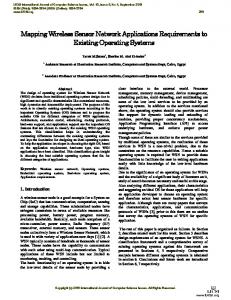
Fig. 9. Segmentation results for miscellaneous shapes and densities. (i) cross: 2200 nodes, average 12 neighbors per node. (ii) cactus: 2100 nodes, average 9 neighbors per node. (iii) airplane: 1900 nodes, average 7.8 neighbors per node. (iv) gingerman: 2700 nodes, average 8 neighbors per node. (v) hand: 2500 nodes, average 6.5 neighbors per node. (vi) single-hole: 3700 nodes, average 13 neighbors per node. (vii) spiral: 2900 nodes, average 11 neighbors per node. (viii) smiley: 2900 nodes, average 8 neighbors per node. (ix) star: 3900 nodes, average 9 neighbors per node.

In Figure 10(i), the green and pink segments are adjacent to each other. Definition 4.2. Adjacency Graph: In an adjacency graph G = (V, E), each segment si is denoted as a vertex vi in V . There is an edge eij ∈ E between vi and vj , if the corresponding two segments si and sj are adjacent to each other. An adjacency graph is showed in Figure 10(ii). An adjacency graph is compact. Its size is proportional to the number of segments, which is a small constant in most scenarios. We construct this adjacency graph by using the nodes on the boundaries of the segments to discover the adjacency information locally. More specifically, the construction contains the following ACM Journal Name, Vol. V, No. N, June 2008.


·

21

two steps: (1) Construct local adjacency graph. Nodes on the boundaries of segments propagate the IDs of the adjacent segments along the flow pointers towards one of the sinks of the sink cluster. Intermediate nodes cache received messages (together with possible extra information, e.g., hop counts to the boundary nodes) for future usage. Messages with the same information can be suppressed if necessary. All sinks further forward the collected information to the sink cluster leader, which only requires one or two hop transmissions since all sinks are close to each other. Eventually, the leader can gather a local picture about what segments are adjacent to itself. (2) Construct global adjacency graph. To get a complete adjacency graph, sink cluster leaders exchange their adjacency information via the shortest paths through segment boundary nodes built up during the first phase. After that, leaders push the global graph down to other nodes inside its segment via reversed flow pointers. We may also augment the adjacency graph with additional useful information on its vertices and edges. For example, if the nodes are aware of their locations, vertices can be associated with the locations of sinks, which will be useful to get a global rough layout; edges can be associated with the Euclidean distance/hop counts between two sinks for finding shortest paths at the top level. In general, we can augment the graph with whatever information gathered by sink nodes, for example, the size of a segment, the number of nodes on the boundary between two segments, etc. These information would aid the design of efficient and load balanced protocols. The above two-phase construction algorithm makes the augmented adjacency graph presented at multiple resolutions at sensor nodes, which will further facilitate the applications. Each node only knows rough information about far-apart segments based on the adjacency graph; but it can store more detailed information about the closest adjacent segments (e.g. the shortest paths to the boundaries). We will elaborate the usage of segmentation together with adjacency graph through various applications in Section 5.

(i)

(ii)

Fig. 10. An example of adjacency graph. (i) An irregular sensor field with four segments; (ii) The corresponding adjacency graph.

ACM Journal Name, Vol. V, No. N, June 2008.

22

·

Xianjin Zhu et al.

5. APPLICATIONS In this section, we present several specific applications that benefit from shape segmentation. These applications are commonly encountered during network design, spanning fundamental problems such as facility placement and routing, as well as data processing, such as data storing and uniform sampling. At the application level, we assume that location information can be made available depending on applications’ requirements. But our shape segmentation scheme runs without any geographical information. In fact, the geographical information only gives a node local picture of its neighborhood, but nodes are still unaware of the global features of the network. Simulation results show that shape segmentation improves performance in terms of efficiency and load balance, and facilitates the selection of protocols and the calibration of protocol parameters. 5.1 Routing in Irregular Networks Multi-hop routing is one of the most fundamental functionalities of all kinds of communication networks. Readers can refer to a survey paper [Al-Karaki and Kamal 2004] to get a comprehensive understanding of routing challenges and protocols in sensor networks. Among the huge literature on routing, geographical routing becomes one of the most popular protocols in sensor networks because it is nearly stateless and avoids message flooding. However, as we mentioned before, inaccurate location information and complex topological features cause geographical routing to have degraded performance in practice. Routing protocols proposed upon virtual coordinate systems [Fang et al. 2005; Bruck et al. 2005] do overcome the above weaknesses, but involve non-trivial design of virtual coordinates dependent on the deployment features. Network segmentation approaches this problem by partitioning the sensor field, so that existing algorithms are still useful inside each segment. It provides a generic recipe for both routing and other applications — inside a segment, existing protocols can still be reused; across segments, an application-dependent structure integrates segment-level data together. Thus, routing and other upper level applications can be conducted in a universal and flexible way. For example, we can choose different protocols for intra-segment and inter-segment routing, purely depending on application requirements. Routing across segments is achieved with the segmentation adjacency graph. Suppose a source node x in segment si wants to send packets to destination y in segment sj . x first finds a desired high level path from si to sj on the adjacency graph by using inter-segment routing. Inside each segment, packets are routed towards the boundary nodes or the destination with intra-segment protocol. The two-level routing scheme follows the philosophy of [Fang et al. 2005]. But the partitioning of the sensor field is done in a different manner. We discuss the details and possible protocols that can be used at these two levels. (1) Inter-segment routing. We use the adjacency graph for global route planning. There can be multiple paths from one segment to the other. In Figure 10, two paths connect the left (green) segment to the right (dark blue) segment. Depending on available augmented information and application requirements, we can use different criteria to choose a desired path. For example, distance information (or hop counts) augmented on edges can be helpful to find the shortest path; the ACM Journal Name, Vol. V, No. N, June 2008.


·

23

number of boundary nodes between two segments implies if there is a bottleneck, which can be used to distribute traffic loads on multiple paths. After selecting a path, packets are forwarded along the set of segments on the path sequentially. (2) Intra-segment routing. Intra-segment routing is used for routing packets between a pair of nodes inside the same segment. Since each segment relatively has a nice shape (i.e., with simple geometry, without holes), most routing protocols proposed in the literature can be directly used for this purpose. We can use geographical routing if location information is available; we can also use landmarkbased routing by simply putting landmarks at the boundaries of the segments. What routing protocol to use inside a segment is totally independent of intersegment routing. Each segment can even choose its own protocol. This gives more flexibility to users. We compare the performance of routing aided by segmentation with GPSR [Karp and Kung 2000] without segmentation. Simulations are conducted on the network showed in Figure 11(i) and Figure 12(i). 10000 source-destination pairs were chosen in each topology. For the topology in Figure 11(i), sources and destinations were selected from either the left segment or the right segment. In the other topology (Figure 12(i)), sources were from the segment at the left-upper corner, and destinations were at the right-bottom corner. We use GPSR combined with manhattan routing4 for intra-segment routing and for inter-segment routing, we distribute traffic to multiple (e.g., 2 paths in both tested topology) high-level routes based on the size of the segments on the path. From the simulations, we found that the path length averaged on 10000 pairs in both network fields are close to GPSR. In the topology of Figure 11(i), segmentationaided routing produces shorter paths than GPSR. Since each segment has relatively nice shape, geographical routing can work well inside segments. Routing along the outer boundary, which happens more frequently in GPSR, is avoided by intersegment routing. Figure 11 and Figure 12 show the load distribution in the networks, which is counted as the number of transmissions incurred at each node. The darker the color, the higher load a node has. It is clear that nodes with higher load are around boundaries without segmentation. With segmentation, more nodes are involved in packet forwarding. Thus, traffic is more evenly distributed among nodes. average path length routing with segmentation GPSR

topology of Fig 11(i) 39.73 49.13

topology of Fig 12(i) 36.38 30.67

Table I. The path length averaged over 10000 source-destination pairs in two different network fields, with and without segmentation.

4 Basically, if a source at (x , y ) wants to transmit packets to a destination at (x , y ). Packets s s d d are first greedily forwarded to the closest node at (xs , yd ) along a roughly vertical path, then that node forwards packets to the destination along a roughly horizontal path, or vice versa.


24

·

Xianjin Zhu et al.

(i)

(ii)

(iii)

Fig. 11. (i) Network topology (ii) Load distribution with segmentation-aided routing. (iii) Load distribution in GPSR without segmentation. Black nodes are with load > 800 transmissions; red nodes are with load > 500 transmissions; green nodes are with load > 300 transmissions; yellow nodes are with load > 100 transmissions

(i)

(ii)

(iii)

Fig. 12. (i) Network topology (ii) Load distribution with segmentation-aided routing. (iii) Load distribution in GPSR without segmentation. Black nodes are with load > 800 transmissions; red nodes are with load > 500 transmissions; green nodes are with load > 300 transmissions; yellow nodes are with load > 100 transmissions.

5.2 Facility Location The problem of base station placement is usually a concern at the very beginning of network design. An intuitive optimization criterion is to place multiple base stations in a way such that the average distance from a sensor to its nearest base station is minimized, so the total energy consumption for data transmissions between sensors and base stations can be minimized. Solutions for the above placement problem can be classified into two categories. One class includes several centralized approaches based on mathematical models (e.g., integer linear programming) [Shi and Hou 2007; Chandra et al. 2004]. Centralized approaches give optimal or near-optimal solutions, but they are not suitable for sensor networks wherein nodes are self-organized and do not have any global knowledge. By observing the similarity between the placement problem and the clustering problem, a second approach adapts existing clustering algorithms (e.g., k-means clustering [MacQueen 1967]) to suggest the placements of base stations. Specifically, in k-means algorithm, k random locations are selected as the cluster centers. Then the rest of the nodes are partitioned into k clusters, with all the ACM Journal Name, Vol. V, No. N, June 2008.


·

25

nodes closest to one center put in the same cluster. Then the centroid of each cluster is picked as the new center and the algorithm iterates until the centers do not move much. Although the adapted clustering algorithms work well in practice, there are a few limitations of those algorithms. —The number of base stations to be placed (parameter k) may depend on the specific deployment of the sensor network, thus is hard to specify before hand. —Typically k random locations are selected as the initial locations in the k-means algorithm. Different initial locations result in different final placement. —The clustering algorithms try to place base stations based on the distances between cluster centers and the rest of the nodes, but do not respect the geometric features of the underlying physical environment. Inside one cluster bottlenecks can still occur. Motivated by the limitations of the existing algorithms, we found that segmentation provides an alternative solution for the placement problem. The number of segments gives a natural choice for k and the set of sinks can be directly replaced by base stations. More important, the segmentation reflects the significant geometric features of a sensor field, and avoids placing a base station to cover two groups of sensors connected by a narrow bridge. To aggregate data from sensors in each segmentation, the aggregation tree has been implicitly constructed during the segmentation phase. Every node can simply follow the flow pointers to forward data to base stations. By aggregating data within each segment first, we can dramatically reduce network traffic through bottlenecks. We compare the average distance (hop counts) between a sensor node and its closest base station under different network topologies. We first test the best k for an irregular sensor field by running the k-means algorithm with different k. Figure 13 shows the average distance from a sensor to its closest base station over k in a cross-shape network field (Figure 9(i)). As the number of base stations increases, the average distance is reduced, but the cost of deployment increases. To be the most cost effective with a reasonable budget, Figure 13 suggests to place 4 ∼ 6 base stations, since the average distance can not be reduced much with more than 6 base stations. This is consistent with the number of segments (5 segments) the segmentation algorithm gives. Thus, in the following comparisons, we only compare the segmentation approach to the k-means algorithm with k equal to the number of segments, which is a good indication of the number of base stations needed. We compare the segmentation approach with k-means algorithm. With segmentation, one solution is to place a base station at the centroid location of the sink cluster at each segment. Each node chooses the base station inside the same segment as its own base station. Furthermore, we combine the segmentation with k-means algorithm by using the centroid location of sink clusters as the initial placement, then running k-means algorithm based on that. The performance of three approaches is showed in Table II. The k-means algorithm with the initial position as the sinks of the segments works the best. One thing worth noticing is that the pure segmentation approach achieves comparable performance compared to k-means algorithm and the combined one, but avoids the cost of multiple iterations required in the k-means algorithm, and more importantly, it suggests a good ACM Journal Name, Vol. V, No. N, June 2008.

26

·

Xianjin Zhu et al.

choice for the parameter k, deciding which is typically a challenge in the standard k-means algorithm. 12 cross Average hops

10 8 6 4 2 0

2

4

6

8

10

k Fig. 13. The average hops from a sensor to its closest base station over various k in a cross-shape network. average hop counts k-means shape segmentation k-means over segmentation

cross 5.02 5.76 4.95

plane 5 5.78 4.94

corridor 7.42 7.83 7.36

fish 11.58 12.01 11.55

Table II. The average hops from a sensor to its closest base station with and without shape segmentation.

5.3 Distributed Index Distributed index for multi-dimensional data (DIM [Li et al. 2003]) is a quadtree type hierarchy that supports efficient multi-resolution data storage and range query. The key idea of DIM is to map an event with certain values to a specific area called as zone, and store the event with geographic routing to the node owning that zone. The zone is determined by dividing the bounding rectangle of the network alternatively with a vertical or horizontal line until there is a single node inside the zone. When a node generates an event, it estimates the destination zone based on the event value and routes it towards there. DIM provides a scalable index structure for data storage and performs well in a network field with simple geometric topology. However, it suffers a lot from load unbalancing in a complex shaped sensor field. For a network with arbitrary shape, there will be large empty space in the bounding rectangle. Some nodes (especially those boundary nodes) must take care of a larger zone, and hence store more data than others. Overloaded nodes would be depleted faster than other nodes, which may lead to network partitioning and shorten network lifetime. With shape segmentation, we can avoid above problems by applying DIM on each segment. Specifically, we first divide the entire event range into several sub-ranges. Let Ni denote the number of nodes belonging to the ith segment, and N denote the ACM Journal Name, Vol. V, No. N, June 2008.


250

250

200

200

150

150

100

100

50

50

0

0

(i)

·

27

(ii)

Fig. 14. (i) Distribution of storage load in basic DIM structure. (ii) Distribution of storage load in shape segmentation integrated DIM structure.

total number of nodes. Sub-ranges are divided based on the ratio of Ni /N . The first segment takes care of events within range [0, N1 /N ), and the second segment takes care of the range [N1 /N, (N1 + N2 )/N ), and so on. A new generated event is divided into several sub-events, each of which is sent towards the corresponding segments respectively. Inside each segment, the sub-event is processed in the same way as the basic DIM algorithm. To compare the performance of DIM with and without shape segmentation, we run simulations on various network scenarios. We generated 10000 events with values uniformly distributed in a fixed range [0, 1000], and stored them into the network. Figure 14 shows the distribution of storage load for the cross network. We can see that the boundary nodes in the basic DIM structure suffer much higher loads than the rest of the network. On the other hand, with shape segmentation, since each segment has tighter bounding rectangle and each node is associated with an almost equal sized zone, data is seen to be well distributed across the network with no particular preference for occurrence of peaks. The peaks in Figure 14(i) reach 248, while the highest peak in Figure 14(ii) is only 65. Shape segmentation also helps reduce communication cost by mapping events into more accurate locations. Table III shows that the average communication cost in terms of hop counts for every event insertion is much less with shape segmentation in all three different network scenarios, viz. cross (Fig. 9(i)), corridor (Fig. 6) and fish network (Fig. 1). In the cross and corridor network, shape segmentation saves 60% ∼ 70% cost. The gain in fish-type network is about 20%, not as significant as the previous two cases. The reason is that each piece of ‘fish’ does not tightly match with its bounding rectangle. cost per event insertion without shape segmentation with shape segmentation

cross 293.69 84.15

corridor 359.21 151.05

fish 254.37 204.58

Table III. Average data insertion cost for DIM with and without shape segmentation.


28

·

Xianjin Zhu et al.

5.4 Random Sampling We discuss the benefits of shape segmentation with another example - random sampling. Uniform random sampling of a sensor node is a fundamental operation that is used as a basic element in many scenarios such as geographical hash tables [Ratnasamy et al. 2002], geographical gossip [Dimakis et al. 2006] and information diffusion and storage [Dimakis et al. 2005]. The basic sampling procedure works as follows [Bash et al. 2004]. A node who wants to pick a random sensor in the network first chooses a random geographical location inside the bounding rectangle, and uses geographical routing to route towards that location. The message will eventually arrive at the node closest to the picked location. A node p is picked with a probability proportional to the area of its Voronoi cell. To achieve a uniform sampling distribution, the acceptance probability of sampling at each node needs to be adjusted, as the one with a large Voronoi cell is more likely to be picked. Basically, each sampled node will be accepted with probability ri = min(τ /ai , 1), where τ is a given threshold and ai is the area of the Voronoi cell associated with node i. If a node rejects a sample, it will pick a new location and repeat the above process. In an irregular sensor field, the Voronoi cells of different nodes have vastly varying areas. Nodes with large Voronoi cells are picked more likely, yet often get rejected afterwards. Thus, the sampling efficiency suffers as a lot of trials end up in vain. Furthermore, since the fate of each sample can only be determined at the destination node, samples may be rejected after traveling a long path, which incurs expensive communication cost and wastes network resources. Random sampling integrated with shape segmentation can dramatically reduce the number of unnecessary trials, at the same time achieving uniform sampling. The adapted algorithm runs as follows. Each time before sampling, we first randomly select a segment. Each segment is selected with probability Pi = Ni /N . After that, we pick a random location within the bounding rectangle of the selected segment. Within each segment we apply the same sampling algorithm and sampling rejection policy as before. Segments are divided into Voronoi cells with much smaller variation, thus no node would reject samples with abnormally high probability. We run simulations on the same three typical networks. Results are averaged on 10 rounds, and in each round, we randomly pick 100 samples. For the basic random sampling algorithm, we set τ to the ratio of the size of the network field and the total number of nodes. Each segment has its own τ as the ratio of the segment size and number of nodes belonging to that segment. In Table IV, we compare the average number of trials taken to get 100 samples. The basic random sampling algorithm tried 168, 149 and 136 times for ‘cross’, ‘corridor’ and ‘fish’ respectively. Shape segmentation reduces the number to 112, 115 and 123. Table V shows the average communication cost per sample. As expected, the cost in shape segmentation case is less than the basic case. With the same observation we got in DIM, shape segmentation shows different levels of improvements in different network scenarios. For these two applications, the performance more or less depends on whether the bounding rectangle is tight enough. We notice that this is due to an inherent assumption of the basic sampling algorithm that uses a bounding rectangle on the sensor field. Further improvement ACM Journal Name, Vol. V, No. N, June 2008.

Segmenting A Sensor Field: Algorithms and Applications in Network Design no. of trials without shape segmentation with shape segmentation

cross 168 112

corridor 149 115

·

29

fish 136 123

Table IV. Average number of trials for 100 random sampling. cost per sampling without shape segmentation with shape segmentation

cross 477.84 102.49

corridor 511.95 182.32

fish 361.80 238.47

Table V. Average cost per sampling.

can be made by using a tighter polygon to approximate the shape of the segment in the basic sampling algorithm. 5.5 Discussion We mainly presented several common problems encountered during network design and management. But the applications of shape segmentation can go beyond that. For example, the recent work on information dissemination and collection by sweeps [Skraba et al. 2006] can be directly integrated with shape segmentation and be applied inside each segment. Shape segmentation can also help the construction of virtual coordinate systems. Take a landmark-based routing scheme [Fang et al. 2005] for an example in which the placement of landmarks has a critical impact on its performance. Since the segments have a nice shape, a few landmarks inside each segment would suffice for routing in and between segments. We summarize the impact of shape segmentation on network design and protocol development: —Segmentation provides, at a global level, a compact way to represent the underlying diverse geometric features of a sensor network field, and makes the network design and protocol development transparent to the specific deployment. —Segmentation facilitates the design and development of new topology-adaptive protocols and makes existing protocols that assume nice shaped field reusable. —Segmentation gives users great flexibility to ‘mix-and-match’ protocols and calibrate important protocol parameters with respect to the specific deployment. 6. CONCLUSION In this paper we introduced a simple distributed algorithm that partitions an irregular sensor field into nicely shaped segments, by using the connectivity information. We show that segmentation is a generic approach to handle complex geometric features and improve the performance of algorithms that assume a nice regular sensor field. We expect that more applications will benefit from this general approach with improved performance in an irregular sensor field. In shape segmentation, a generally unsolved issue is that there is no well accepted definition on good segmentation so far. The choice of appropriate segmentation may also depend on the applications. For example, a spiral-like sensor field is equivalently nice as a long corridor for routing protocols, but it needs to be segmented ACM Journal Name, Vol. V, No. N, June 2008.

30

·

Xianjin Zhu et al.

further for applications that require a quad-tree type hierarchy. We proposed two schemes to give certain guarantees on the fatness of the segments but also provide flexibility for the upper level applications to pick a definition and choose proper segmentation granularity. One interesting problem is to classify applications into several categories so that more precise segmentation definitions can be found for each category. We regard this as our future work. ACKNOWLEDGMENTS

We thank Yue Wang for sharing with us the boundary detection code in [Wang et al. 2006] and Alexander Kröller for a few useful discussions. This work is partially supported by NSF CAREER Award CNS064387 and funding from the Center of Excellence in Wireless and Information Technology, Stony Brook University. REFERENCES Al-Karaki, J. N. and Kamal, A. E. 2004. Routing techniques in wireless sensor networks: a survey. IEEE Wireless Communications 11, 6, 6–28. Bash, B. A., Byers, J. W., and Considine, J. 2004. Approximately uniform random sampling in sensor networks. In DMSN ’04: Proceeedings of the 1st international workshop on Data management for sensor networks. ACM Press, New York, NY, USA, 32–39. Bose, P., Morin, P., Stojmenovic, I., and Urrutia, J. 2001. Routing with guaranteed delivery in ad hoc wireless networks. Wireless Networks 7, 6, 609–616. Bruck, J., Gao, J., and Jiang, A. 2005. MAP: Medial axis based geometric routing in sensor networks. In MobiCom ’05: Proceedings of the ACM/IEEE International Conference on Mobile Computing and Networking. 88–102. Chandra, R., Qiu, L., Jain, K., and Mahdian, M. 2004. Optimizing the placement of integration points in multi-hop wireless networks. In ICNP ’04: Proceedings of International Conference on Network Protocols. 271–282. Choi, H. I., Choi, S. W., and Moon, H. P. 1997. Mathematical theory of medial axis transform. Pacific Journal of Mathematics 181, 1, 57–88. Dey, T. K., Giesen, J., and Goswami, S. 2003. Shape segmentation and matching with flow discretization. In WADS ’03: Proceedings of workshop on Algorithms and Data Structures. 25–36. Dimakis, A. G., Prabhakaran, V., and Ramchandran, K. 2005. Ubiquitous access to distributed data in large-scale sensor networks through decentralized erasure codes. In IPSN ’05: Proceedings of the fourth international symposium on information processing in sensor networks. 111–117. Dimakis, A. G., Sarwate, A. D., and Wainwright, M. J. 2006. Geographic gossip: efficient aggregation for sensor networks. In IPSN ’06: Proceedings of the fifth international conference on Information processing in sensor networks. ACM Press, New York, NY, USA, 69–76. Elson, J. 2003. Time synchronization in wireless sensor networks. Ph.D. thesis, University of California, Los Angeles. Fang, Q., Gao, J., Guibas, L., de Silva, V., and Zhang, L. 2005. GLIDER: Gradient landmarkbased distributed routing for sensor networks. In INFOCOM ’05: Proceedings of the 24th Conference of the IEEE Communication Society. Vol. 1. 339–350. Fang, Q., Gao, J., and Guibas, L. J. 2006. Landmark-based information storage and retrieval in sensor networks. In The 25th Conference of the IEEE Communication Society (INFOCOM’06). 1–12. ¨ ller, A., Pfisterer, D., Fischer, S., and Buschmann, C. 2004. Fekete, S. P., Kro Neighborhood-based topology recognition in sensor networks. In ALGOSENSORS. Lecture Notes in Computer Science, vol. 3121. Springer, 123–136. ACM Journal Name, Vol. V, No. N, June 2008.


·

31

Funke, S. 2005. Topological hole detection in wireless sensor networks and its applications. In DIALM-POMC ’05: Proceedings of the 2005 Joint Workshop on Foundations of Mobile Computing. ACM Press, New York, NY, USA, 44–53. Funke, S. and Klein, C. 2006. Hole detection or: ”how much geometry hides in connectivity?”. In SCG ’06: Proceedings of the twenty-second annual symposium on Computational geometry. ACM Press, New York, NY, USA, 377–385. Funke, S. and Milosavljevic, N. 2007. Network sketching or: ”how much geometry hides in connectivity?–part ii”. In SODA ’07: Proceedings of the Eighteenth Annual ACM-SIAM Symposium on Discrete Algorithms. 958–967. Ganeriwal, S., Kumar, R., and Srivastava, M. B. 2003. Timing-sync protocol for sensor networks. In SenSys ’03: Proceedings of the 1st international conference on Embedded networked sensor systems. ACM Press, New York, NY, USA, 138–149. Greenstein, B., Estrin, D., Govindan, R., Ratnasamy, S., and Shenker, S. 2003. DIFS: A distributed index for features in sensor networks. In Proceedings of First IEEE International Workshop on Sensor Network Protocols and Applications. 163–173. Hilaga, M., Shinagawa, Y., Kohmura, T., and Kunii, T. L. 2001. Topology matching for fully automatic similarity estimation of 3d shapes. In SIGGRAPH ’01: Proceedings of the 28th annual conference on Computer graphics and interactive techniques. ACM Press, New York, NY, USA, 203–212. Karp, B. and Kung, H. 2000. GPSR: Greedy perimeter stateless routing for wireless networks. In MobiCom ’00: Proceedings of the ACM/IEEE International Conference on Mobile Computing and Networking. 243–254. ¨ ller, A., Fekete, S. P., Pfisterer, D., and Fischer, S. 2006. Deterministic boundary Kro recognition and topology extraction for large sensor networks. In Proceedings of 17th ACMSIAM Sympos. Discrete Algorithms. 1000–1009. Kuhn, F., Wattenhofer, R., Zhang, Y., and Zollinger, A. 2003. Geometric ad-hoc routing: Of theory and practice. In PODC ’03: Proceedings of 22 nd ACM Int. Symposium on the Principles of Distributed Computing. 63–72. Leymarie, F. F. and Kimia, B. B. 2001. The shock scaffold for representing 3d shape. In Proceedings of 4th International Workshop Visual Form. 216–228. Li, X., Kim, Y. J., Govindan, R., and Hong, W. 2003. Multi-dimensional range queries in sensor networks. In Proceedings of the first international conference on Embedded networked sensor systems. ACM Press, 63–75. Lieutier, A. 2003. Any open bounded subset of Rn has the same homotopy type than its medial axis. In SM ’03: Proceedings of the eighth ACM symposium on Solid modeling and applications. ACM Press, 65–75. MacQueen, J. B. 1967. Some methods for classification and analysis of multivariate observations. In Proceedings of 5-th Berkeley Symposium on Mathematical Statistics and Probability. 281– 297. Ratnasamy, S., Karp, B., Yin, L., Yu, F., Estrin, D., Govindan, R., and Shenker, S. 2002. GHT: A geographic hash table for data-centric storage in sensornets. In Proc. 1st ACM Workshop on Wireless Sensor Networks ands Applications. 78–87. Sebastian, T., Klein, P., and Kimia, B. 2001. Recognition of shapes by editing shock graphs. In ICCV ’01: Proceedings of International Conference on Computer Vision. 755–762. Shi, Y. and Hou, Y. T. 2007. Approximation algorithm for base station placement in wireless sensor networks. In SECON ’07: Proceedings of IEEE Communications Society Conference on Sensor and Ad Hoc Communications and Networks. 512–519. Siddiqi, K., Shokoufandeh, A., Dickinson, S. J., and Zucker, S. W. 1998. Shock graphs and shape matching. In ICCV ’98: Proceedings of International Conference on Computer Vision. 222–229. Skraba, P., Fang, Q., Nguyen, A., and Guibas, L. 2006. Sweeps over wireless sensor networks. In IPSN ’06: Proceedings of the fifth international conference on Information processing in sensor networks. ACM Press, New York, NY, USA, 143–151. ACM Journal Name, Vol. V, No. N, June 2008.

32

·

Xianjin Zhu et al.

Wang, Y., Gao, J., and Mitchell, J. S. B. 2006. Boundary recognition in sensor networks by topological methods. In MobiCom ’06: Proceedings of the ACM/IEEE International Conference on Mobile Computing and Networking. 122–133.


Segmenting A Sensor Field: Algorithms and Applications in Network

Segmenting A Sensor Field: Algorithms and Applications in Network

Suggest Documents

Sensor Network Applications - Diku.edu

WIRELESS SENSOR NETWORK APPLICATIONS

Underwater Sensor Network Applications: A Comprehensive Survey

Developing and Deploying Sensor Network Applications ... - CiteSeerX

Wireless Sensor Network - Theoretical Findings and Applications

Wireless Sensor Network - Theoretical Findings and Applications

Survey on Wireless Sensor Network Applications and

Wireless Sensor Network Applications: A Study in ... - Science Direct

Developing Wireless Sensor Network Applications in a ... - CiteSeerX

Sensor Network Applications in Structures â A Survey

Sensor network routing algorithms for realistic

SENSOR REGISTRATION IN A SENSOR NETWORK BY ...

A Survey of Wireless Sensor Network Applications From a Power ...

Prototyping Wireless Sensor Network Applications with BTnodes

Sensor Network Applications - University of Southampton

Building Distributed Sensor Network Applications ...

Outline for Sensor Network Workplaces Applications - CiteSeerX

Wireless Sensor Network Applications for Healthcare - ijacta

Sensor Network Applications - University of Southampton

Implementing Wireless Sensor Network Applications ... - IEEE Xplore

Prototyping Wireless Sensor Network Applications with BTnodes

Mapping Wireless Sensor Network Applications Requirements to ...

Research on the Algorithms for Registration in Sensor Network for ...

Efficient Algorithms for Segmenting Globally ... - Semantic Scholar

Segmenting A Sensor Field: Algorithms and Applications in Network