e c o l o g i c a l m o d e l l i n g 2 2 0 ( 2 0 0 9 ) 589–594
available at www.sciencedirect.com
journal homepage: www.elsevier.com/locate/ecolmodel
Short Communication
Selecting pseudo-absence data for presence-only distribution modeling: How far should you stray from what you know? Jeremy VanDerWal a,∗ , Luke P. Shoo a , Catherine Graham b , Stephen E. Williams a a
Centre for Tropical Biodiversity and Climate Change, School of Marine and Tropical Biology, James Cook University, Townsville, Queensland 4811, Australia b Department of Ecology and Evolution, 650 Life Sciences Building, Stony Brook University, NY 11794, USA
a r t i c l e
i n f o
a b s t r a c t
Article history:
An important decision in presence-only species distribution modeling is how to select back-
Received 18 September 2008
ground (or pseudo-absence) localities for model parameterization. The selection of such
Received in revised form
localities may influence model parameterization and thus, can influence the appropriate-
5 November 2008
ness and accuracy of the model prediction when extrapolating the species distribution
Accepted 18 November 2008
across time and space. We used 12 species from the Australian Wet Tropics (AWT) to evaluate the relationship between the geographic extent from which pseudo-absences are taken and model performance, and shape and importance of predictor variables using the MAXENT
Keywords:
modeling method. Model performance is lower when pseudo-absence points are taken from
AUC
either a restricted or broad region with respect to species occurrence data than from an inter-
Conservation
mediate region. Furthermore, variable importance (i.e., contribution to the model) changed
Model evaluation
such that, models became increasingly simplified, dominated by just two variables, as the
Pseudo-absence data
area from which pseudo-absence points were drawn increased. Our results suggest that
Species distribution model
it is important to consider the spatial extent from which pseudo-absence data are taken. We suggest species distribution modeling exercises should begin with exploratory analyses evaluating what extent might provide both the most accurate results and biologically meaningful fit between species occurrence and predictor variables. This is especially important when modeling across space or time—a growing application for species distributional modeling. © 2008 Elsevier B.V. All rights reserved.
1.
Introduction
Appropriate selection of pseudo-absence or background locations is essential for presence-only species distribution modeling (SDM) (Chefaoui and Lobo, 2008). Recent studies have highlighted several methods for selection of pseudo-
∗
absence points including at: random (e.g., Stockwell and Peters, 1999); random with geographic-weighted exclusion (e.g., Hirzel et al., 2001); random with environmentally weighted exclusion (e.g., Zaniewski et al., 2002); locations that have been visited (i.e., occurrences for other species) but where the target species was not recorded (e.g., Elith
Corresponding author. Tel.: +61 7 47815570; fax: +61 7 47251570. E-mail addresses:
[email protected],
[email protected] (J. VanDerWal). 0304-3800/$ – see front matter © 2008 Elsevier B.V. All rights reserved. doi:10.1016/j.ecolmodel.2008.11.010
590
e c o l o g i c a l m o d e l l i n g 2 2 0 ( 2 0 0 9 ) 589–594
and Leathwick, 2007); and occurrences for an entire group of species collected using the same methods, encapsulating sampling bias of data (e.g., Phillips and Dudik, 2008). While the relative merits of these different methods have been discussed previously (e.g., Lütolf et al., 2006; Chefaoui and Lobo, 2008; Phillips and Dudik, 2008), one important methodological step that has not been properly evaluated is the extent of the geographic region in which background or pseudo-absence points are taken. We suspect that, in practice, the decision to set spatial constraints on the background is typically one that is made unconsciously. Modelers simply default to using the extent of an arbitrarily defined study area. But does this really matter? There are several reasons why pseudo-absences selected at large distances from known occurrences may be problematic. Essentially, pseudo-absences are meant to provide a comparative data set to enable the conditions under which a species occurs to be contrasted against those where it is absent. If pseudo-absences are geographically disparate from the presence locations, predictive models will be dominated by parameters that serve to coarsely discriminate regional conditions with weakened ability to tease out fine scale conditions that actually limit the species distribution. This is in direct conflict with the purpose of generating pseudoabsences in the first place. The objective of this study was to ask whether background size really matters and, if so, how far from presence localities should selection of pseudo-absence points be taken? We address both questions by selecting random pseudo-absences from increasingly larger background areas and monitoring the impact this has on the predictions of species distribution models. Specifically, we examine 12 rainforest vertebrates
from the Australian Wet Tropics (AWT) and employ a common presence-only ecological niche modeling methodology, MAXENT (Phillips et al., 2006). In this application MAXENT is used to represent both background and pseudo-absence modeling. We explore changes in model accuracy, predicted distributional area and relative importance of predictor variables with increasing background size.
2.
Methods
The AWT of northeastern Australia is an ideal candidate region for testing our objectives (Fig. 1). The region contains a diverse, well-studied vertebrate fauna and encompasses strong environmental gradients. The AWT supports 1.8 million ha of rainforest-dominated vegetation that was once widespread in Miocene Australia but now forms a distinct and isolated environmental domain of high diversity surrounded by drier and warmer environments (Nix, 1991; Moritz, 2005). We modeled vertebrate species across different taxonomic groups with varying degrees of environmental specialization and range size. The species (and number of occurrences in brackets) examined included: mammals—Melomys cervinipes (230), Pseudochirops archeri (169) and Dendrolagus bennettianus (17); birds—Meliphaga lewinii (707), Amblyornis newtonianus (144) and Oriolus flavocinctus (158); reptiles—Morelia kinghorni (199), Lampropholis robertsi (36) and Saproscincus lewisi (13); and frogs—Litoria genimaculata (489), Cophixalus hosmeri (89) and Cophixalus infacetus (162). Species environmental specialization, range size and occurrences (collected during extensive field surveys and collated from the literature and institutional databases) are described in Williams (2006).
Fig. 1 – Backgrounds from which pseudo-absences were drawn for C. hosmeri and predicted distributions in the Australia Wet Tropics region (outlined in black) given the different background sizes. Increasing background size corresponds to darkening of buffering bands surrounding the occurrence points of the species (represented as x symbols here) in the left image; these regions represent increasing distances from 10 to 500 km from the occurrence points. Warmer colors on the right images infer greater predicted suitability for the C. hosmeri. Grey areas fall below the threshold of suitability and are assumed to not be part of the distribution.
e c o l o g i c a l m o d e l l i n g 2 2 0 ( 2 0 0 9 ) 589–594
The environmental data used for the modeling included four climatic variables; mean annual temperature, maximum temperature of the warmest month, annual precipitation and precipitation of the driest quarter. Spatial climate layers for current climate were estimated using the Anuclim 5.1 software (McMahon et al., 1995) and an ∼250 m resolution DEM (GEODATA 9 Second DEM Version 2; Geoscience Australia, http://www.ga.gov.au/). All distribution models were created using a maximum entropy algorithm (MAXENT ver. 3.2.1) (Phillips et al., 2006). This algorithm is increasingly being employed to model species’ distributions. MAXENT has been shown to perform well in comparison to other algorithms (Elith et al., 2006; Hernandez et al., 2006). For all models created, we used default settings in MAXENT as outlined in Phillips and Dudik (2008). The only parameter that we varied among models, for each species, was the size of the background (i.e., study region) from which pseudo-absences were selected. In each case models were trained on 10,000 pseudo-absence points drawn at random from a background whose area was defined using incrementally increasing distances from occurrence points (distance bands of 10, 25, 50, 75, 100, 150, 200, 300, 400, and 500 km as depicted in Fig. 1). We used the area under the curve (AUC) test statistic calculated in two different ways to evaluate the impact of
591
background size on model performance (as per Phillips and Dudik, 2008). First, we calculated AUC using pseudo-absences taken from the entire background used to build the model, hereafter referred to as ‘flexible area AUC’. Second, we calculated AUC for a fixed evaluation area comprising ∼36,000 points representing a 1 km grid across the AWT, herein termed ‘fixed area AUC’. Here, the same pseudo-absences were used for all models regardless of the spatial extent of training data. This enabled us to correct for any bias in test statistics that may have been introduced by varying the background size itself. Note that the AWT is an intermediate size, ∼36,000 km2 , in relation to the distance bands used to generate background regions. We also quantified change in the relative importance of environmental variables as a function of increased background size. Analyses included comparisons of flexible area AUC, fixed area AUC and proportion of AWT predicted as suitable distribution area across background sizes ranging from 10 to 500 km and predictor variable importance. The predicted distribution area was estimated by applying a “balance” threshold that minimized 6 × training omission rate + .04 × cumulative threshold + 1.6 × fractional predicted area. This threshold was selected as it was consistently ranked the best for these species using the expert opinion of Stephen E. Williams (James Cook University, Townsville, Australia) and Luke P. Shoo (James Cook University, Townsville, Australia).
Fig. 2 – Comparisons of model statistics (flexible area and fixed area AUC), proportion of Australia Wet Tropics (AWT) predicted as part of the species distribution and relative contributions of environmental variables to models for all species examined (see Section 2 for an explanation of flexible area and fixed area AUC).
592
3.
e c o l o g i c a l m o d e l l i n g 2 2 0 ( 2 0 0 9 ) 589–594
Results
The results are summarized in Fig. 2. Model predictions and performance changed in at least four important ways as the area of the background from which pseudo-absences were drawn increased. First, the flexible area AUC increased. Specifically, the AUC increased rapidly as background size expanded from 10 to 100 km. Subsequent expansions resulted in only minor increases in AUC (i.e., at 100 km all models already had an AUC > 0.93 and by 500 km AUC > 0.99). Second, in 50% of the species, the fixed area AUC declined gradually. For the remaining cases the fixed area AUC underwent an initial increase across background sizes up to 100–200 km before then conforming to the general pattern of decline observed in the other species. Third, variable importance (i.e., contribution to the model) changed. Essentially, models became increasingly dominated by just two variables (maximum temperature of the warmest period and precipitation of driest quarter). Fourth, in general, the proportion of the fixed area predicted to be suitable for a species increased. Interestingly, however, for almost half of the species, the overall increase was initially preceded by a sharp decrease in predicted area for background sizes up to 100 km. The pattern was particularly evident in C. hosmeri shown also Fig. 1.
4.
Discussion
Here we show that the size of background from which pseudo-absences are drawn has important ramifications for predictions and performance of SDMs. We have focused on predictions of current distributions but this issue will likely be even more problematic for models that are projected onto different geographic space or under different climate scenarios. For example, inappropriate background selection may unduly affect studies of invasive species (e.g., Mau-Crimmins et al., 2006; Steiner et al., 2008) or attempts to predict past and future distributions (e.g., Hilbert and Ostendorf, 2001). We show that pseudo-absences drawn from too small an area can produce spurious models while pseudo-absences drawn from too large of an area can lead to artificially inflated test statistics and predictions of distribution area as well as potentially less informative response variables. Such errors will be propagated when projecting onto the novel environmental space, potentially providing misleading results. Larger training backgrounds were coupled with higher flexible area AUC values (Fig. 2, top left). However, we interpret this simply as an artifact of the method used to derive the test statistic. That is, occurrences and pseudo-absences are more likely to be classified correctly when pseudo-absences are drawn at greater distances from known occurrences that contain vast areas of unsuitable environment for the species. The usefulness of AUC as a model test statistic for SDM has previously been questioned (see e.g., Lobo et al., 2008). While it is not our intention to reiterate the reasons here, we do acknowledge that some limitations of the AUC test statistic are exemplified in our training data. To correct for the particular inconsistency introduced by varying background size, we also calculated AUC for a fixed evaluation area where the
same pseudo-absences were used for all models regardless of the spatial extent of training data. This permitted internally consistent comparisons of models created for each species. In doing so, we find that, for the 12 species taken together, AUC was maximized at a background size of about 200 km. For many species, models performed poorly at smaller background sizes and there was a gradual decline in AUC for all species at when points were generated from larger regions (Fig. 2, top right). Variables identified as being important predictors in SDMs are thought to be useful in generating mechanistic hypotheses about parameters governing distributions. However, we find that variable importance is itself strongly affected by background size (Fig. 2, bottom right). Models became more simplified with increasing background size and were increasing dominated by just two variables. Resulting distributions more closely resembled the broad extent of rainforest rather than suitable habitat for a particular species (e.g., C. hosmeri, Fig. 1). Put simply, increasingly simplified models were dominated by variables that provided good regional discrimination (Australia Wet Tropics versus surrounding drier, warmer environment) but failed to identify more subtle changes in suitability over finer scale gradients likely to be under selection by the species being modeled. Concomitant with this result, we found that finer scale resolution of predicted habitat (i.e., distinct fragments and complex boundaries) was lost (see Fig. 1) and predicted distribution area increased (Fig. 2, bottom left) as the area from which pseudo-absences were generated increased. These characteristics have important implications for modeling applications. After all, conservation priorities at regional scales are often already known given broad species ranges; finer resolution of boundaries at the scale of individual habitat patches is exactly what is demanded from the SDM exercise in order to set conservation goals (i.e., identifying specific locations to include in reserve systems) (Harris et al., 2005). Further, extent of occurrence and area of occupancy are two parameters that are widely employed to determine the conservation status of species (e.g., IUCN, 2001 criteria). As such, artificially inflated estimates of distribution area by using pseudo-absences selected from an inappropriate background, for example, may have the potential to unduly influence the outcomes of such assessments. Our results complement previous findings by Thuiller et al. (2004) who suggested that there is an optimal distance in environmental space (as opposed to geographic space) from which pseudo-absences should be selected for estimation of current and future species distributions. The authors reported spurious projections given pseudo-absences drawn from environmental space too similar to that of the occurrences. At the other extreme, models trained using pseudo-absences drawn from as broad environmental space as possible resulted in liberal over-predictions. Further, pseudo-absences selected from inappropriate locations distorted response curves (as described by Thuiller et al., 2004) with additional affects expected for predicted distribution size, validation statistics and the contribution of parameters to predictive models, as we have shown here. Some of the implications of pseudo-absence selection can be seen in other studies. For example, Growns and West
e c o l o g i c a l m o d e l l i n g 2 2 0 ( 2 0 0 9 ) 589–594
(2008) classified aquatic bioregions for conservation using overlapping distributions of fish species predicted from SDMs. Pseudo-absences were selected from the entirety of New South Wales, Australia (an area larger than our 500 km buffer). In doing so, the authors inadvertently demonstrated several key results described here. Individual species’ distributions were found to exhibit “substantial to almost perfect model accuracy”. However, the result is arguably due to the fact that test statistics simply evaluated the ability of the models to discriminate between a restricted set of occurrences and pseudo-absences drawn from vast areas of unsuitable environment space. We also expect that resultant models represent over-predictions of the true potential species distributions with only regional discrimination rather than refined predictions of actual species’ distributions—a result that aided in the goals of the study. The findings of our analysis on background size introduce yet another source of uncertainty into the presence-only SDM exercise. This is in addition to biases and errors that arise from inaccuracies in the occurrence or environmental data, parameter choice or idiosyncrasies of different model algorithms (see e.g., Araújo and New, 2007). However, like many of these issues, we argue that the problem of selecting an appropriate background size is not an insurmountable one. With proper consideration, the issue can be adequately managed in modeling applications. Foremost, we need to be aware that background size has the potential to impact model predictions and performance. We then need to explicitly vary background size and monitor for change in test statistics, variable importance and prediction area. Armed with this information we can then make sensible decisions about what constitutes an appropriate background. For our data, we conclude that 200 km was an “optimal” distance to stray in search of appropriate pseudo-absence points. This essentially represented a compromise between producing models that did not generalize well (i.e., response curves were only generated across a small subset of possible environmental conditions) and producing inflated estimates of model performance and over predictions of distribution area that ignored important spatial structure associated with finer scale gradients. We now encourage other researchers to pursue similar exercises with their data and report findings so that we might eventually be able to make prescriptions for background selection that will work in most applications.
Acknowledgements This research was supported by the James Cook University Research Advancement Program, the Marine and Tropical Sciences Research Facility, Earthwatch Institute and the Queensland Smart State Program.
references
Araújo, M.B., New, M., 2007. Ensemble forecasting of species distributions. Trends Ecol. Evol. 22, 42–47.
593
Chefaoui, R.M., Lobo, J.M., 2008. Assessing the effects of pseudo-absences on predictive distribution model performance. Ecol. Model. 210, 478–486. Elith, J., Graham, C.H., Anderson, R.P., Dudik, M., Ferrier, S., Guisan, A., Hijmans, R.J., Huettmann, F., Leathwick, J.R., Lehmann, A., Li, J., Lohmann, L.G., Loiselle, B.A., Manion, G., Moritz, C., Nakamura, M., Nakazawa, Y., Overton, J.M., Peterson, A.T., Phillips, S.J., Richardson, K., Scachetti-Pereira, R., Schapire, R.E., Soberon, J., Williams, S., Wisz, M.S., Zimmermann, N.E., 2006. Novel methods improve prediction of species’ distributions from occurrence data. Ecography 29, 129–151. Elith, J., Leathwick, J., 2007. Predicting species distributions from museum and herbarium records using multiresponse models fitted with multivariate adaptive regression splines. Divers. Distrib. 13, 265–275. Growns, I., West, G., 2008. Classification of aquatic bioregions through the use of distributional modelling of freshwater fish. Ecol. Model. 217, 79–86. Harris, G.M., Jenkins, C.N., Pimm, S.L., 2005. Redefining biodiversity conservation priorities. Conserv. Biol. 19, 1957–1968. Hernandez, P.A., Graham, C.H., Master, L.L., Albert, D.L., 2006. The effect of sample size and species characteristics on performance of different species distribution modeling methods. Ecography 29, 773–785. Hilbert, D.W., Ostendorf, B., 2001. The utility of artificial neural networks for modelling the distribution of vegetation in past, present and future climates. Ecol. Model. 146, 311– 327. Hirzel, A.H., Helfer, V., Metral, F., 2001. Assessing habitat-suitability models with a virtual species. Ecol. Model. 145, 111–121. IUCN, 2001. IUCN Red List Categories and Criteria: Version 3.1. IUCN Species Survival Commission. IUCN, Gland, Switzerland/Cambridge, UK. Lobo, J.M., Jimenez-Valverde, A., Real, R., 2008. AUC: a misleading measure of the performance of predictive distribution models. Glob. Ecol. Biogeogr. 17, 145–151. Lütolf, M., Kienast, F., Guisan, A., 2006. The ghost of past species occurrence: improving species distribution models for presence-only data. J. Appl. Ecol. 43, 802–815. Mau-Crimmins, T.M., Schussman, H.R., Geiger, E.L., 2006. Can the invaded range of a species be predicted sufficiently using only native-range data? Lehmann lovegrass (Eragrostis lehmanniana) in the southwestern United States. Ecol. Model. 193, 736–746. McMahon, J.P., Hutchinson, M.F., Nix, H.A., Ord, K.D., 1995. ANUCLIM User’s Guide, Version 1. Centre for Resource and Environmental Studies, Australian National University, Canberra, 90 pp. Moritz, C., 2005. Overview: rainforest history and dynamics in the Australian Wet Tropics. In: Bermingham, E., Dick, C.W., Moritz, C. (Eds.), Tropical Rainforests. University of Chicago Press, Chicago, pp. 313–322. Nix, H., 1991. Biogeography: pattern and process. In: Nix, H.A., Switzer, M.A. (Eds.), Rainforest Animals: Atlas of Vertebrates Endemic to Australia’s Wet Tropics. Australian National Parks and Wildlife, Canberra, pp. 11–40. Phillips, S.J., Anderson, R.P., Schapire, R.E., 2006. Maximum entropy modeling of species geographic distributions. Ecol. Model. 190, 231–259. Phillips, S.J., Dudik, M., 2008. Modeling of species distributions with Maxent: new extensions and a comprehensive evaluation. Ecography 31, 161–175. Steiner, F.M., Schlick-Steiner, B.C., VanDerWal, J., Reuther, K.D., Christian, E., Stauffer, C., Suarez, A.V., Williams, S.E., Crozier, R.H., 2008. Combined modelling of distribution and niche in invasion biology: a case study of two invasive Tetramorium ant species. Divers. Distrib. 14, 538–545.
594
e c o l o g i c a l m o d e l l i n g 2 2 0 ( 2 0 0 9 ) 589–594
Stockwell, D., Peters, D., 1999. The GARP modelling system: problems and solutions to automated spatial prediction. Int. J. Geogr. Inf. Sci. 13, 143–158. Thuiller, W., Brotons, L., Araújo, M.B., Lavorel, S., 2004. Effects of restricting environmental range of data to project current and future species distributions. Ecography 27, 165–172. Williams, S.E., 2006. Vertebrates of the Wet Tropics Rainforests of Australia: Species Distributions and Biodiversity. Cooperative
Research Centre for Tropical Rainforest Ecology and Management. Rainforest CRC, Cairns, Australia, 282 pp. Zaniewski, A.E., Lehmann, A., Overton, J.M., 2002. Predicting species spatial distributions using presence-only data: a case study of native New Zealand ferns. Ecol. Model. 157, 261–280.