Distribution modeling and simulation of gene expression data

Computational Statistics and Data Analysis 53 (2009) 1650–1660

Contents lists available at ScienceDirect

Computational Statistics and Data Analysis journal homepage: www.elsevier.com/locate/csda

Distribution modeling and simulation of gene expression data Rudolph S. Parrish a,∗ , Horace J. Spencer III b , Ping Xu a a Department of Bioinformatics and Biostatistics, School of Public Health and Information Sciences, University of Louisville, 555 S. Floyd St, Suite 4026, Louisville,

KY 40292, USA b Department of Biostatistics, College of Public Health, University of Arkansas for Medical Sciences, West Markham St., Little Rock, AR, USA

article

info

Article history: Available online 29 March 2008

a b s t r a c t Data derived from gene expression microarrays often are used for purposes of classification and discovery. Many methods have been proposed for accomplishing these and related aims, however the statistical properties of such methods generally are not well established. To this end, it is desirable to develop realistic mathematical and statistical models that can be used in a simulation context so that the impacts of data analysis methods and testing approaches can be established. A method is developed in which variation among arrays can be characterized simultaneously for a large number of genes resulting in a multivariate model of gene expression. The method is based on selecting mathematical transformations of the underlying expression measures such that the transformed variables follow approximately a Gaussian distribution, and then estimating associated parameters, including correlations. The result is a multivariate normal distribution that serves to model transformed gene expression values within a subject population, while accounting for covariances among genes and/or probes. This model then is used to simulate microarray expression and probe intensity data by employing a modified Cholesky matrix factorization technique which addresses the singularity problem for the “small n, big p” situation. An example is given using prostate cancer data and, as an illustration, it is shown how data normalization can be investigated using this approach. © 2008 Elsevier B.V. All rights reserved.

1. Introduction In high-dimensional gene expression microarray systems, one of the important problems facing investigators concerns development of new statistical methods (or efficient application of existing methods) to achieve aims of classification or discovery. One might wish to classify an individual patient’s disease so that the patient’s therapy could be tailored for maximal efficacy, for example. Determining which genes play a role in the disease is a process of discovery involving microarrays as a screening tool. Another, less often discussed, objective is to monitor disease progression or recovery subsequent to diagnosis or treatment. Gene expression relates to protein synthesis and metabolic parameters in a systems biology context, so that characterization at the level of the gene is useful in focusing subsequent efforts, such as investigating gene regulatory networks and pathways. Ultimately, one needs to reduce the vast information contained in microarrays, and perhaps other relevant clinical parameters, to a relatively simple form which permits its practical use. Statistically, this includes characterizing the data as succinctly as possible without losing information content. Mathematical and statistical modeling methods can be applied advantageously to help address these aims. If microarray data can be modeled accurately, statistical methods can be examined with respect to their relative usefulness in applications. This includes various methods relating to significance testing for differences between groups and identification of differentially expressed genes. While

∗ Corresponding author. Tel.: +1 502 852 2797; fax: +1 502 852 3294. E-mail address: [email protected] (R.S. Parrish). 0167-9473/$ – see front matter © 2008 Elsevier B.V. All rights reserved. doi:10.1016/j.csda.2008.03.023

R.S. Parrish et al. / Computational Statistics and Data Analysis 53 (2009) 1650–1660

1651

there are several proposed methods for doing this, there is very little information about the performance characteristics of such methods when applied to microarray data. In experiments involving different subjects (or, equivalently, multiple independent samples), there is natural subject-tosubject variation that occurs for expression levels of all genes (usually termed “biological variation”), and there is natural variation that occurs when multiple arrays are utilized within the same subject which can be due to sampling error or other factors. Variation among subjects is the basis for the experimental error term used in significance testing. That is, the subject generally is considered as being the experimental unit. Other situations could involve multiple samples derived longitudinally from the same subject (e.g., time-course experiments). Systematic or “technical” variation also often exists in relation to the experimental design or other aspects of conducting the experiment. Singhal et al. (2003) developed a microarray data simulator in which systematic and random technical variability and biological variability were added onto a model of underlying gene expression. Nykter et al. (2006) developed a modular model involving sources of variation that included slide manufacturing, biological noise, hybridization, and scanning error; this model requires specification of a large number of parameters. Albers et al. (2006) provided a web page for simulation of two-channel cDNA arrays. While addressing underlying sources of variation, none of these approaches incorporated correlations among genes, and all relied on multiple assumptions. In the course of investigating properties of various methods, many other authors (e.g., Molinaro et al. (2005)) have used simulation approaches typically based on the multivariate normal distribution with fixed, simplified covariance structures. In reality, the covariance matrix does not follow a simple structure, nor do the marginal distributions follow a normal or even lognormal model. Thus, something more realistic is needed. In this paper, a method is proposed in which variation among arrays (usually one array per biological unit) can be characterized simultaneously for a large number of genes resulting in a multivariate model of gene expression, which incorporates both biological and technical variation. The emphasis is on characterizing the true nature of the array data without pre-specification or presumption of an underlying, unknown ‘ground truth’, as other methods typically require. In some contexts, the ‘ground truth’ can be thought of as the parent multivariate distribution model that gives rise to the data. It is possible to incorporate treatment effects and other sources of variation if the application requires it. The proposed method is based on selecting mathematical transformations of the underlying expression measures such that the transformed variables follow approximately a Gaussian (i.e., normal) distribution, and then estimating associated parameters, including correlations (or covariances). The result of this procedure is a multivariate normal distribution that serves to model the transformed gene expression values among subjects and takes into account correlations among genes. The same approach can be used to characterize underlying probe-level intensity data, incorporating correlations also among probes within genes. This approach makes it possible to simulate gene expression and probe intensity data enabling an investigator to produce arbitrarily large sample sizes so that properties of different statistical methods can be evaluated and compared. This includes normalization, classification (Xu et al., 2009), and differential-expression testing algorithms. Another potential use is in development of numerical indices that relate to disease progression and recovery when disease status is assessed longitudinally. With this approach, epidemiologically derived gene expression data can be summarized for populations of interest to be used as reference groups. In addition to use of gene expression data, this approach also makes it possible to include clinically derived information for continuously measured variables and their correlations with gene expressions. In any given situation, subsets of genes can be modeled using the corresponding joint distribution derived from the complete model fit, thus enabling detailed analyses of genes of interest, as for example those in some defined pathway. In the following, we first describe the methodology for fitting the multivariate model and subsequently generating random array data. We then evaluate the method by comparing various aspects of simulated data to the training data, particularly as regards the goodness of fit to the empirical distributions and the capability to reproduce correlations among genes and probes. The results are based on application to data derived from a study of prostate cancer patients. An example of applying this methodology to the problem of data normalization is presented for illustration.

2. Methods r 2.1. Affymetrix GeneChip technology

Technical aspects of oligonucleotide arrays have been discussed in several publications (Affymetrix, 2002; Nguyen et al., r 2002). In brief, GeneChip arrays provide information on gene expression by measuring multiple probe intensities, each consisting of 25-mer base pairs or more, depending on the version of the array design, which then are utilized in one of many available algorithms to produce composite measures of gene expression. The Human U95Av2 array contains a grid of 640 × 640 probes grouped in 12,525 sets, with each set consisting of 11–20 probe pairs (median 16), and with each set corresponding to a single gene transcript. Some microarrays map multiple probe sets to individual genes. Commonly employed expression algorithms, which include Microarray Suite 5.0 (MAS 5.0) (Affymetrix, 2002), Robust Multiarray Average (RMA) (Irizarry et al., 2003), and dChip (Li and Wong, 2001), mathematically process probe-level data to produce gene-specific expression values.

1652

R.S. Parrish et al. / Computational Statistics and Data Analysis 53 (2009) 1650–1660

2.2. Multivariate normal distribution model In order to develop a multivariate distribution model of gene expression, expression data are examined for each gene individually using an automated algorithm to select a transformation that produces approximately a Gaussian (i.e., normal) probability distribution. For purposes of this discussion, arrays are assumed to be independently associated with individual subjects, although generalization to multiple arrays within subjects is straightforward. For each gene, a transformation is determined on the basis of data from all subjects in a particular category, such as healthy subjects or patients with disease. After making all appropriate transformations for the entire set of genes under study, the means, variances, and covariances (between pairs of genes) of transformed variables are estimated. Thus, a multivariate Gaussian distribution model is constructed having as density function the general form: f (z; µ, 6 ) = (2π)−p/2 |6|−1/2 exp{−0.5(z − µ)0 6 −1 (z − µ)}, −∞ < zi < ∞, where z is the vector of transformed variables, µ is the vector of means of the transformed variables, and 6 is the matrix of variances and covariances of the transformed variables. In essence, this process involves selecting appropriate transformations that result in marginal distributions of the transformed variables which are approximately Gaussian. An important property of this model is that any subset of the transformed variables also has a multivariate normal distribution with corresponding parameters taken directly from µ and 6 . In addition, there are closed-form relations for determining the corresponding variance–covariance matrix in the case where conditional distributions are of interest (Morrison, 1976; Johnson and Kotz, 1972). This means that subsets of genes are automatically modeled as soon as the overall model is fully specified, so that genes which may be related to each other as a result of a common gene regulatory network or pathway can be considered independently of other genes. 2.3. Transformations to normality Based on our extensive empirical investigations, no single transformation family can provide the scope of transformations necessary to obtain a high percentage of good approximations to the data, as measured by a goodness-of-fit criterion. Often a simple lognormal transformation is employed as a normalizing transformation, but it fails to provide adequate fits in a substantial proportion of cases, sometimes for as much as 70% of the data. In order to find a best fitting distribution, two types of normalizing transformation families were considered: (1) Box–Cox power transformation (Box and Cox, 1964) and (2) Johnson transformation system (Johnson and Kotz, 1970). Both of these are nonlinear methods and may require iterative algorithms for implementation. The Johnson system includes the lognormal distribution. The Box–Cox transformation was recently considered by Giles and Kipling (2003) for use with microarray data. Some modifications to this method have been proposed (see Sakia (1992), for a review and bibliography, and also Kirisci et al. (2005)), however the original transformation was used here. In our work, an empirical approach to fitting was adopted in which each possible transformation was applied to each gene’s data (across subjects) and the Kolmogorov–Smirnov (KS) goodness-of-fit (GOF) statistic was used to identify the best fitting transformation in each case. These transformations should be considered as mechanisms to achieve approximate normality. They are essentially four-moment transformations, thus issues of overfitting are not of concern. For example, with the Johnson system, skewness and kurtosis can be used to define which member of the family is selected for modeling a marginal distribution. In a diagram presented in Johnson and Kotz (1970), the lognormal distribution corresponds to a curved line in the skewness–kurtosis plane, which implies that the family of distributions is much richer than the lognormal distribution allows, and hence distribution modeling is more likely to succeed. After transformation, all that is needed for the multivariate model are the means, variances, and covariances, as well as the limits of variation for some distributions. With the Box–Cox family, a single parametric transformation is employed but requires an iterative approach. In any given case, a distribution from either family could be better than the other. (1) Box–Cox transformation. The traditional Box–Cox family of transformations is defined by y = (xθ − 1)/θ, if θ 6= 0, and y = log(x), if θ = 0, where θ is a parameter selected to achieve normality and where x is the original (i.e., untransformed) expression value of a given gene transcript, as described above. Estimation of θ is based on maximization of the correlation coefficient between the x- and y-values of a standard normal probability plot. Computationally, an optimal value of θ can be found by an iterative search process. (2) Johnson system of distributions. The Johnson system of distributions is defined on the basis of three transformations; these are denoted by: SL (lognormal), SB (bounded), and SU (unbounded). In addition, a null transformation is denoted here by SN , where the subscript denotes √ “normal”. This system uniquely associates a distribution with each possible pair of values of skewness ( β1 ) and kurtosis √ 3/2 (β2 ), the standardized third and fourth moments ( β1 = µ3 /µ2 and β2 = µ4 /µ22 , where µr represents the rth central moment). That is, each possible pair of skewness and kurtosis values is associated with a unique distribution in the Johnson system. Possible (β1 , β2 ) values are restricted to the region β2 ≥ β1 + 1 (Johnson, 1987). The normal distribution has fixed skewness and kurtosis coefficients equal to 0 and 3, respectively, and this is represented as a single point in the skewness–kurtosis plane. The lognormal distribution has skewness and kurtosis coefficients that are related according to the parametric equations β1 = (ω − 1)(ω + 2)2 and β2 = ω4 + 2ω3 + 3ω2 − 3 where ω = exp(η2 ) with η2 being the variance of the log-transformed variable. Thus, in the (β1 , β2 ) plane, these equations define a curved line that divides the possible pairs of values. On one side of this line, corresponding to kurtosis lower than for lognormal (for fixed skewness),

R.S. Parrish et al. / Computational Statistics and Data Analysis 53 (2009) 1650–1660

1653

are points corresponding to SB distributions; while the other side corresponds to SU distributions and has kurtosis higher than for the lognormal. As the Johnson system of distributions includes combinations of skewness and kurtosis that are far different from the lognormal, it provides a much wider variety of normalizing transformations than are available with the log transformation alone. A good approximation is more likely to be found using the Johnson system than if the lognormal distribution were used exclusively. Letting x represent a gene expression variable, a standardizing transformation for location and scale may be applied in the form: (x − ξ)/λ where ξ and λ are constants. For the SL distribution, the value of λ may be taken to be 1 without loss of generality; and thus ξ is the lower terminus of the three-parameter lognormal distribution. For the SB distribution, λ will be the range of variation, λ = B − A where A < x < B, and ξ = A is the lower limit of variation. The Johnson normalizing transformations, as given by Rose and Smith (2002), are defined as: SL : y = log(x − ξ),

ξ < x < ∞, SB : y = log[(x − ξ)/(ξ + λ − x)], ξ < x < (ξ + λ), [(x − ξ)/λ] = log[(x − ξ)/λ + {1 + [(x − ξ)/λ]2 }1/2 ],

(1) (2)

−1

SU : y = sinh

−∞ < x < ∞,

(3)

and SN : y = (x − ξ)/λ,

−∞ < x < ∞.

(4)

Further define z = γ + δy where the parameters γ and δ control the shape of the distribution. In each case, parameter values are sought so that Z has a standard normal distribution. Thus, this system involves four parameters: ξ, λ, γ , and δ. For estimation purposes, let µ = −γ/δ and σ = 1/δ. These correspond to the mean and standard deviation of Y for one of the four transformations, as the case may be. With these definitions, y = µ + σ z. 2.4. Estimation of means, variances, and covariances Methods using iterative techniques are available for estimating the parameters of the distributions based on the Box–Cox and some members of the Johnson transformations (Rose and Smith, 2002; Johnson, 1949, 1965; Johnson and Kitchen, 1971; Zhou and McTague, 1996). For the Johnson system, methods based on percentiles have been described by Wheeler (1980), Slifker and Shapiro (1980), Bowman and Shenton (1989), and Shayib (1989). The method of moments also may be used in some cases. Although each method proposed for transforming to normality has advantages, none seems to be clearly superior, especially considering the variability seen among the large number of genes involved. Thus, an empirical approach is taken here for obtaining a best fitting normal approximation in which the KS GOF statistic is used as the fitting criterion. Each of the approaches described below is employed in turn and the corresponding numerical value of the KS statistic is obtained. The final selection of a transformation and the associated parameter estimates correspond simply to the minimumvalued KS statistic that is observed. This is done for each gene so that the end result is a table containing designations of the type of transformations and the associated parameter estimates. (a) Box–Cox transformation: An initial value for the parameter θ in the Box–Cox formulation is obtained by a systematic search over the interval [−3,3] in equal steps (e.g., 15 values). For each such value, the Box–Cox transformation is made, moment estimates are used for the normal distribution parameters, and the KS GOF statistic D is evaluated. The two smallest consecutive values of D determine an interval that contains the θ value which produces the minimum D. A binary search algorithm is then employed to converge on the optimal solution for θ, in which each step requires that the transformation be made, distribution parameters be estimated, and the GOF criterion D be computed. Throughout this procedure, if the absolute value of θ is less than a specified small tolerance value, such as 0.05, the log transformation is applied rather than the power transformation. At each step, after the Box–Cox transformation is done, the sample mean (m1 ) and standard deviation (m2 ) for the transformed values are computed, which are used to compute the parameter estimates: γ ∗ = −m1 /m2 and δ∗ = 1/m2 . (b) Johnson system: Selection of an appropriate Johnson distribution may be based on the third and fourth standardized moments (i.e., skewness and kurtosis), followed by an iterative approach for estimating distribution parameters for the selected type. The large number of genes and potential numerical problems make this approach difficult to implement reliably, especially since higher-order moments are more difficult to estimate with small sample sizes. Although the choice of distribution type can be based on the skewness and kurtosis values, anomalies in the data that translate to variability in moment estimates sometimes make it difficult to pick reliably the best fitting approximation using this method. Owing to these factors, the selection and fitting process for Johnson distributions employs both the method described by Slifker and Shapiro and an empirical-based ad hoc approach as described below. Slifker–Shapiro fitting method: The method of Slifker and Shapiro (1980) is based on the use of four equally spaced points from the transformed standard normal distribution, denoted by −3z, −z, z, and 3z. When z = 0.524, for example, this corresponds to the 70th percentile and 3z = 1.572 corresponds to the 94.2th percentile. Different values of z may be more desirable for use with small data sets, such that 3z is not at the extreme quantiles of the empirical data. The empirical percentiles are derived from the raw data by calculating the cumulative standard normal probabilities for these four points (denoted by P−3z , P−z , Pz , and P3z ) and then inferring the corresponding raw values using the ith order statistic of the raw data where

R.S. Parrish et al. / Computational Statistics and Data Analysis 53 (2009) 1650–1660

1654

i = NP + 0.5, with N being the sample size. Interpolation is used when i is not an integer. These empirical percentiles are denoted by x−3z , x−z , xz , and x3z . Letting m = x3z − x−z , n = x−z − x−3z , and p = xz − x−z , the following ratios determine the

type of Johnson distribution: SU : mn/p2 > 1, SB : mn/p2 < 1, and SL : mn/p2 = 1. As the SL ratio is unlikely ever to be exactly equal to unity, a tolerance interval around 1 is used to permit selection of the lognormal. (For this analysis, a tolerance of 0.05 was used.) Then, the distribution parameters are estimated using the closed-form formulas given by Slifker and Shapiro. Empirical fitting method: In the empirical fitting method, a GOF-based procedure is applied for each gene individually and for each of the Johnson distributions separately. After all distribution types have been optimally fitted in this fashion, the one which has the smallest KS GOF statistic is selected as the best fitting Johnson distribution. The steps are as follows: 1. Select one of the Johnson distribution transformations. 2. Determine initial values A and B to represent the range of possible values for X . The absolute limits for A are 0 to xmin , and for B are xmax to 216 − 1 (or 16 if a log-base-two transformation is made to the raw intensity values). The following initial values are suggested: A = Xmin − tol∗ (xmax − xmin ) and B = Xmax + tol∗ (xmax − xmin ) for some pre-specified tolerance value, such as 0.05. 3. Apply the following procedure for the current values of A and B: (a) Set ξ = A and λ = B − A, and compute y-values as given above for the selected transformation. (b) Calculate the sample mean (m1 ) and standard deviation (m2 ) of these transformed values for each gene, to be used as moment estimators of the normal distribution parameters. (c) Compute the one-sample KS GOF test statistic, D, used in assessing normality. 4. Vary the tolerance value over a defined range, such as 0.01 to 0.09, and modify the values of A and B until an optimum value for the goodness-of-fit statistic is achieved for each distribution type. The effect of this is to determine values for A and B corresponding to each distribution separately such that the KS statistic is minimized. 5. Select the transformation corresponding to the smallest value of D for each gene. 6. Compute the sample mean (m1 ) and standard deviation (m2 ) for the selected transformation values (y). These optionally can be based on robust procedures such as trimmed moments. 7. The parameter estimates (denoted by *) then are given by: ξ∗ = A, λ∗ = B − A, γ ∗ = −m1 /m2 , δ∗ = 1/m2 . For simplicity of fitting, ξ is taken as the lower limit of variation of x and ξ + λ is taken as the upper limit, although these may not be optimal choices due to the transformations involved. While this procedure is not statistically optimal, it performs adequately for the purpose of selecting and fitting a distribution as an approximation to the underlying true distribution, and it can be performed efficiently in the context of a large number of genes. A more refined approach involving estimation of ξ and λ can be implemented but, then, four sample moments are required for estimation rather than two and a nonlinear optimization algorithm must be employed in which numerical convergence is not guaranteed. 2.5. Simulation of gene expression data Random deviates from a multivariate normal distribution can be generated easily using a triangular factorization of the variance–covariance matrix, provided such a factorization exists. Particularly, if the covariance matrix 6 can be factored as 6 = TT0 where T is a lower triangular matrix and if u represents a vector of standard normal independent random deviates, then y = µ + Tu defines a vector of random deviates from the desired multivariate normal distribution, having the desired covariance structure. In this representation, µ is the mean vector for the transformed variables (y) and 6 is the covariance matrix for the transformed variables. The Cholesky decomposition algorithm (Kennedy and Gentle, 1980) may be used to obtain T when 6 is positive definite. With microarray data, however, 6 usually will be only positive semi-definite, owing to the large number of genes under consideration relative to the number of arrays (experimental units). In this case, a modified Cholesky algorithm may be employed to obtain T (Schnabel and Eskow, 1990, 1991, 1999) which, in effect, modifies 6 so that it is positive definite. The modifications are generally minimal. After generating standard normal deviates using the matrix transformation above, conversion to original scaling is accomplished using inverse transformations for the marginal distributions, which produces random deviates on the original scale. For the Johnson distributions, the inverse transformations are derived algebraically from the transformations given above (Rose and Smith, 2002):

ξ + ey , SB : x = [ξ + (ξ + λ)ey ]/(1 + ey ),

(5)

SL : x =

(6)

SU : x =

ξ + λ sinh(y) = ξ + λ[e − e ]/2,

SN : x =

ξ + λy,

y

−y

(7)

and where y = (z − γ)/δ. For the Box–Cox case, the inverse transformations are: x = (1 + θy) where y = (z − γ)/δ.

(8) 1/θ

, if θ > 0, and x = e , if θ = 0, y

R.S. Parrish et al. / Computational Statistics and Data Analysis 53 (2009) 1650–1660

1655

2.6. Modeling probe-level data Notwithstanding computational limitations, probe-level data can be modeled using the same approach as described above for expression data. However, the dimension of the numerical problem is increased by a factor of 11–16 which may limit the number of genes that can be so represented. It is possible to reduce the requirement for extremely high dimensions by utilizing a nested modeling approach (not discussed here).

2.7. Simulation of differential expression A nominal experiment may be simulated using two treatments, N subjects per treatment, and one array per subject, replicated M times. Treatment effects may be introduced based on an assumed p-value distribution, perhaps a mixture of uniform and beta distributions described by Allison et al. (2002). In order to simulate differentially expressed genes, a p value is generated randomly from the mixture distribution for each gene, and the corresponding t quantile is computed. Under the assumption that a t test would be conducted to test for differential expression, a constant c can be determined and then added to each of the gene expression or probe intensity values in one of the treatment groups, so that the same empirical t value would be obtained had the modified data been used in the calculation. This assumes that the mean or median of the intensity values in each probe set is used as the summary measure of gene expression when simulating probe-level data. This process may be applied before or after background correction and/or normalization of the parent data.

2.8. Computer resources To obtain a benchmark on computing (i.e., CPU) time, 500 arrays were simulated using 4200 genes on a dual-processor 2 GHz Windows XP system with 4 GB RAM. Approximately 49 min of CPU time were required for completion, with about 25% of the time being spent on distribution fitting and about 75% on factorization of the covariance matrix and generation of multivariate normal data. Using a single node on a 64-bit Linux cluster parallel system with dual processors and 4 GB of memory per node, arrays with 12,625 genes have been successfully simulated.

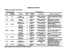
3. Results In this section, we describe a real data set and model it using the foregoing proposed method. After generating simulated data from the fitted model, we compare various aspects of the simulated data to the real data in order to show that the simulated data adequately represent the important features in the parent data set. These include consideration of the following: (1) goodness-of-fit statistics which should show a high percentage of very good fits to the marginal distributions; (2) quantiles (i.e., percentiles) of the real and simulated distributions which should match closely, as shown by quantile–quantile plots; (3) distributions of pair-wise correlations among genes and probes of the real and simulated data which should match closely; and (4) multidimensional scaling components of the real and simulated data which should be similar. Criterion (1) will ensure that the fits to the data for each gene or probe are adequate overall with a high proportion of closely fitting approximations. This can be seen in a cumulative distribution plot of the goodness-of-fit statistics. Criterion (2) will establish that the percentage points, taken over genes and or probes, compare favorably, showing consistency over all genes and/or probes, especially for the tail areas of the distributions. Criterion (3) will ensure that gene- and/or probespecific correlations are closely approximated, indicating that the multivariate model for covariance is reasonable. Criterion (4) will show that the underlying structure of the data is preserved. Establishing all of these criteria will provide strong evidence that the simulated data have the same characteristics as the real data. 3.1. Data from a study in prostate cancer Singh et al. (2002) described a study in which data were collected on prostatectomy patients with specimens being collected both from tumors and adjacent non-tumor prostate tissue (hereinafter called “normal” samples). There were 50 normal and 52 tumor samples, with 47 total paired samples. Expression profiles were derived using oligonucleotide microarrays (H95Av2) containing 12,525 genes. Data files were acquired from the authors’ web site. Raw probe-level data were accessed in the form of “CEL” files produced by Affymetrix analysis software. Those data were processed using R code from the Bioconductor software package module AFFY (Bioconductor, 2003) in order to produce expression values utilizing methods analogous to those employed by Affymetrix MAS 5.0 software. The reason for this approach was that Affymetrix MAS 5.0 output values were available only to one decimal place, which proved insufficient for the purpose of fitting distributions. Model adequacy was assessed and effects of normalization were considered in order to demonstrate utility of the methodology.

1656

R.S. Parrish et al. / Computational Statistics and Data Analysis 53 (2009) 1650–1660

Fig. 1. Scatter plot of quantiles (0.01, 0.05, 0.10, 0.25, 0.50, 0.75, 0.90, 0.95, 0.99) for original and simulated data based on MAS 5.0 expression values for 1000 genes.

Fig. 2. Scatter plot of quantiles for original and simulated data for PM probes (left panel) and PM & MM probes combined (right panel).

3.2. Assessing model adequacy The modeling and simulation procedures described above were applied to the data from normal tissue samples for three cases: (1) MAS 5.0 gene expression values, (2) individual PM probe intensities, and (3) individual PM and mismatch (MM) probe values. For analysis (1), 1000 genes were selected randomly. For probe-based analyses, case (2) used 200 genes with 16 PM probes each (i.e., 3200 probe values), and case (3) used 100 genes having 16 PM and 16 MM probes (i.e., 1600 PM and 1600 MM probe values). The success of the proposed modeling approach was examined for each of these cases by considering goodness-of-fit (GOF) statistics, distribution quantiles, and pair-wise correlations. Simulated data involved 500 arrays. For case (1), the cumulative distribution functions (CDF) of KS GOF statistics show that 98% of the gene distributions were fitted with a KS GOF criterion of less than 0.125, which is acceptable when using the Gaussian distribution to approximate an underlying distribution. Results for other cases were similar. For expression data, approximately 15%, 32%, 1%, 1%, and 52% of the cases were fitted with SU , SB , lognormal, normal, and Box–Cox distributions, respectively. For probe intensity data, these were 13%, 32%, 20%,