Selecting Representative Examples and Attributes by a ... - CiteSeerX
Recommend Documents
ology is validated by showing that program-input pairs that are close to each ..... emit-rtl and insn-emit have a high I-cache miss rate, a low branch prediction ...
cluster borders: partial cluster overlap is better defined. This is in contradiction ..... The second row uses the same fraction ratios as in the selection set (set 1), but ...
Agents's Competition for Selecting a. Representative. Guillermo De Ita, Mireya Tovar, Meliza Contreras. Computer Sciences Faculty, Universidad Autónoma de ...
with an integrated sampling technique, which combines both .... 351. 35. 65. 34 nursery. 12960. 2. 98. 8 thyroid. 215. 13. 87. 5 tic-tac-toe. 958. 34. 66. 9 wine.
Arthur F. Lutz, a,b* Herbert W. ..... skill scores are derived based on earlier work by Perkins et al. (2007) ... temperature, the approach by Perkins et al. (2007) is ...
education, Lego Mindstorms, project based learning, educational technology. 1 Introduction ... robotic turtles which could be programmed with Logo. In our days ...
Silviu Ionita4, Javier Arlegui5, Alfredo Pina5, Emanuele Menegatti6, Michele Moro6,. Nello Fava7, Stefano Monfalcon7, Irene Pagello8. (1) Dept. of Philosophy ...
Andy Georges. Koen De Bosschere ..... Andy Georges is supported by the SEESCOA project spon- sored by the ... [11] M. Martonosi, A. Gupta, and T. Anderson.
Takemove from s10 over s7 to s3 kind man side white. WIN(white) ? LOSS(red). LOSS(red). Normalmove from s2 to s6 kind king side red. Takemove from s10.
Apr 27, 2011 - since the overwhelming majority of new sequences derive from ... genomes and deal exclusively with those. ..... sequences against RP15 (purple), RP35 (orange), RP55 (blue) and RP75 (red) or UniParc (green solid lines).
all html tags and attributes with examples pdf. all html tags and attributes with examples pdf. Open. Extract. Open with
ded in a conceptual framework to guide the application of visualization in knowledge ..... in other settings than just the traditional computer desktop environment.
in relation to statistical methods used for analysing data, it might be more ... O Inter-Research 1995. Resale of full article not permitted .... when some species are removed to a supplementary list. Hellinger distance. This distance between 2 ...
service is a service of unbreakable functionality. On the other hand, a composite service consists of a number of atomic services to constitute a complex service.
Nimrod/G, LSF and so forth), but we cannot introduce all of them in this paper. Finally, we .... needed RAM and HDD, average time needed for execution, approximate execution ... Date, Time and Size of the last successfully finished job (LSJ).
Department Of Computer. Islamic Azad University, ilam branch. Ilam, Iran. Reza Azmi [email protected]. Department Of Computer. Alzahra University. Tehran ...
Rong Fu,Meihong Shi,Hongli Wei,Huijuan chen,"fabric defect detection based on adaptive local binary patterns",international conference on robotics & bi ...
in relation to statistical methods used for analysing data, it might be more efficient to discard rare species from subsequent analyses. In quantitative analysis,.
Jan 25, 2013 - the loan amount offered to a wind farm developer. (Tindal 2011). ... http://www.windnavigator.com/index.php/cms/pages/faq.] Barthelmie, R. J. ... Monaghan, A. J., D. L. Rife, J. O. Pinto, C. A. Davis, and J. R.. Hannan, 2010: ...
Select the paraffin-embedded tumor block with the greatest amount of invasive
carcinoma ... C. A pathologist at Genomic Health will review the H&E slide and, ...
that when learning to recognize a new object (like an apple) we also know a ..... of the apple detector. database [4] to extract examples of common office objects.
Supporting figures S1-S10: Representative examples of aberrant transcription profiles in several candidate genes with U12-processed introns in cases (IGHD ...
Prague University of Economics, Faculty of Management, Jarošovská 1117/II, Jindrichuv Hradec, 37701, Czech Republic [email protected]. Keywords: Feature ...
affinity maturation. However, some proteins. (e.g. T cell receptor) which cannot be dis- played on phage have been successfully dis-. Selecting by microdialysis.
Selecting Representative Examples and Attributes by a ... - CiteSeerX
examples, and of the set of attributes, without impaired classification accuracy. The algorithm ..... For the two genetic algorithms, GA-RK and GA-KJ, Table 4 shows what percentage ..... www.cs.caltech.edu/~muresan/GANN/report.html. Nene, S.
Selecting Representative Examples and Attributes by a Genetic Algorithm Antonin Rozsypal Center for Advanced Computer Studies University of Louisiana in Lafayette Lafayette, LA 70504-4330 [email protected] and Miroslav Kubat Department of Electrical and Computer Egineering University of Miami 1251 Memorial Drive, Coral Gables, FL 33124-0640 [email protected] Abstract A nearest-neighbor classifier compares an unclassified object to a set of preclassified examples and assigns to it the class of the most similar of them (the object’s nearest neighbor). In some applications, many pre-classified examples are available and comparing the object to each of them is expensive. This motivates studies of methods to remove redundant and noisy examples. Another strand of research seeks to remove irrelevant attributes that compromise classification accuracy. The paper suggests to use the genetic algorithm to address both issues simultaneously. Experiments indicate considerable reduction of the set of examples, and of the set of attributes, without impaired classification accuracy. The algorithm compares favorably with earlier solutions.
The input of our algorithm consists of pairs, [~x, c(~x)], where the vector ~x = (x 1 , . . . , xN ) describes the example and c(~x) is its class label. The vector’s elements, xi , are called attributes. When classifying an object, ~y , the nearest-neighbor classifier assigns it the class label of the example with the smallest geometrical distance from ~y . The idea was first put forward by Fix & Hodges (1951) and the first rigorous analysis of its performance was offered by Cover & Hart (1967). The notoriously high classification costs of nearest-neighbor classifiers can be cut down either by indexing techniques or by selecting the most representative examples. The most popular indexing techniques is that of the k-d trees invented by Friedman, Bentley & Finkel (1977) and later improved by Sproull (1991). Another useful spacepartitioning technique was introduced by Nene & Nayar (1997)—see their paper for a summary of other work in this field. Algorithms that select the most representative examples seek to remove those that appear to be noisy or redundant. After the pioneering work by Hart (1968), many alternative solutions have been proposed. Some of them adopt a batch approach, weeding out examples that are noisy or redundant with respect to the entire database. This is the case of the mechanisms developed by Gates (1972), Wilson (1972), Ritter et al. (1975), Tomek (1976), Cortez & Vapnik (1995), Wilson & Martinez (1997), and Kubat & Cooperson (2000). On the other hand, incremental techniques take one example at a time and consider its merit only with respect to the examples that have been seen so far—Aha, Kibler & Albert (1991), Zhang (1992), Cameron-Jones (1995), and Alpaydin (1997). For the sake of completeness, let us mention that a third approach prefers to replace the set of examples with artificially created ones, tuned to the needs of the application at hand. This can be exemplified by the work of Llor`a & Garrell (2001) and by the learning vector quantizer invented by Kohonen (1990). Equally important is the choice of relevant attributes. In a situation where the engineer has no idea which attributes serve best, one may want to describe the examples by as many attributes as can be obtained. However, such perfectionism can be counterproductive. Langley & Iba (1993) showed that the number of examples needed to warrant given classification accuracy grows exponentially in the number of irrelevant attributes and experimental studies carried out by Aha (1990) and other authors corroborate this result. One of the most popular attribute-selecting algorithms, WINNOW, was published by Littlestone (1988). For a survey of alternative methods, see Blum & Langley (1997), where also useful definitions of “relevance” are offered. Knowing that the two-fold problem just described can be cast as a search for the ideal choice of examples and attributes, we wanted to find out whether the popular genetic algorithm (Goldberg, 1989) can be employed. Its versatility is known to be
2
useful particularly in domains where simpler search techniques, such as hill-climbing, suffer from local extremes of the state-evaluation function. We are not the first to pursue this idea. Whereas a technique that employs genetic algorithms to select representative examples was published by Muresan (1997), the question of how to use the approach for attribute selection was investigated as early as by Siedlecki & Sklansky (1989). However, we are only aware of one attempt to use genetic algorithms to address both of these issues simultaneously (Kuncheva & Jain, 1999). A preliminary version of the algorithm we report here was published in our recent conference paper (Rozsypal & Kubat, 2001). Here, we describe a modified version that differs from its predecessor in three aspects: (1) in the way the individual solutions are encoded in chromosomes; (2) in the formula used as fitness function to calculate the survival chances of each solution; and (3) in the use of a more appropriate distance metric that enables to calculate distances between pairs of vectors with non-numeric attributes. Experimental results indicate that this algorithm compares favorably with the solution proposed by Kuncheva and Jain (1999).
2
Description of the Technique
The genetic algorithm (GA) operates with a population of alternative solutions. In the GA terminology, each of the solutions is called a specimen.. For our needs, a specimen will be a subset of examples described by a subset of attributes. Each specimen has a certain value of the fitness function that the approach, taking inspiration from the darwinian evolution principle, seeks to maximize. Concrete implementations of this paradigm differ by the mechanisms they use to encode the specimens as “chromosomes,” by the fitness function, and by the recombination and mutation operators that create a new generation from the older set of specimens. The success or failure of the endeavor also depends on the size of the population and on the criteria to terminate the search. Let us briefly discuss each of these aspects in a separate subsection.
2.1
Chromosomes
In the approach pursued by Kuncheva & Jain (1999), each specimen is represented by a binary chromosome, with each bit representing one of the original training examples and attributes. For instance, if the original number of examples is 1,000 and the number of attributes is 50, then the chromosome will have 1,050 binary alleles. The value “1” indicates that the corresponding example/attribute is to be used and “0” means that it is to be ignored.
3
SPECIMEN:
chromosome 1
chromosome 2
examples
attributes
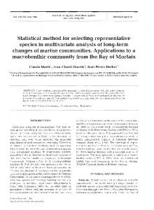
Figure 1: Each specimen is described by two chromosomes, one representing the selected examples and the other representing the selected attributes. The recombination operator (crossover) is applied to each of them separately.
As this encoding may be impractical in domains with many training examples, we opted for the more flexible variable-length scheme where each allele contains an integer that points to a training example or to an attribute. GA literature usually refers to this mechanism as value encoding. Following this approach, we represented each specimen by two chromosomes, one pointing to the chosen examples and the other pointing to the chosen attributes. For instance, the specimen [3,14,39],[2,4] represents a triplet consisting of the third, the fourteenth, and the thirty-ninth training example (all other examples being ignored) described by the second and by the fourth attribute (all other attributes being ignored). When a specimen thus described is used as a classifier, the system selects the examples determined by the first chromosome, and describes them by the attributes determined by the second chromosome. The examples are then employed by the nearestneighbor classifier. The distances between vectors x = (x1 , . . . xn ) and y = (y1 , . . . , yn ) are calculated using the formula: D(x, y) =
q
Σni=1 d(xi , yi )
(1)
where d(xi , yi ) is the contribution of the ith dimension. For numeric attributes, this contribution is calculated as d(xi , yi ) = (xi −yi )2 ; for boolean attributes and for discrete attributes, we define d(xi , yi ) = 0 if xi = yi and d(xi , yi ) = 1 if xi 6= yi .
2.2
Fitness Function
The fitness function quantifies the survival chances of individual specimens. Recall that we want to reduce the number of examples and the number of attributes without compromising classification accuracy in the process. These requirements may contradict each other: in noise-free domains, the entire training set tends to give higher 4
classification performance than a reduced set; likewise, removing attributes is hardly beneficial if each of them provides relevant information. The involved trade-offs are reflected in fitness-function parameters that give the user the chance to specify his or her preferences. The fitness function should make it possible to place emphasis either on maximizing the classification accuracy or on minimizing the number of the retained training examples and attributes. This is the case of the following formula where ER is the number of training examples misclassified by the given specimen, NE is the number of retained examples, and NA is the number of retained attributes. f = 1/(c1 ∗ ER + c2 ∗ NE + c3 ∗ NA )
(2)
Note that the fitness of a specimen is high if its error rate is low, if the set of retained examples is small, and if many attributes have been eliminated. The function is controlled by three user-set parameters, c1 , c2 , and c3 , that weigh the user’s preferences. For instance, if c1 is high, emphasis is placed on classification accuracy; if c2 or c3 are high, emphasis is placed on minimizing the number of retained examples or the number of retained attributes, respectively.
2.3
Choice of Parents and Recombination
From a population of specimens, the genetic algorithm creates a new population by repeatedly picking pairs of “parents,” from which “children” are created by a process called recombination. Parents are selected probabilistically—the following formula is used to calculate the probability that the specimen S’ will be chosen: f (S 0 ) P rob(S 0 ) = P f (S)
(3)
Here, f (S) is the fitness of specimen S as calculated by Equation 2. The denominator sums up the values of the fitness functions of all specimens in the population—this makes the probabilities sum up to 1. A specimen with a high value of the fitness function gets a higher chance of leaving offspring. Once a pair of parents have been chosen, their chromosomes are recombined by a two-point crossover operator to give rise to a pair of children. Let the length of one parent’s chromosome be denoted by N1 and let the length of the other parent’s chromosome be denoted by N2 . Using the uniform distribution, the algorithm selects one pair of integers from the closed interval [1, N1 ] and another pair of integers from the closed interval [1, N2 ]. Each of these pairs then defines a substring in the respective chromosome (the first allele and the last allele are included in the substring). The crossover operator then exchanges the substring from the first chromosome with the 5
Figure 2: The “crossover” operator exchanges randomly selected substrings of parent chromosomes.
substring from the second chromosome. Note that, as each of these substrings can have a different size, the children’s lengths are likely to be different from the parents’ lengths. The process is applied separately to the chromosome containing the list of examples and to the chromosome containing the list of attributes. The principle is illustrated by Figure 2 where the middle parts of chromosomes A and B have been exchanged. Note how the lengths of A and B are affected. Our implementation permits that, in one extreme, the exchanged segments can have size 0 or, in the other extreme, a segment can be identical to a parent.
2.4
Mutation
The mutation operator prevents degeneration of the population’s diversity and makes sure that the population represents a sufficiently large part of the search space. Otherwise, the search process could easily get trapped in a local extreme of the fitness function. Our mutation operator randomly selects a prespecified percentage of the alleles in the newly created population and adds to each of them a random integer generated separately for each allele. The algorithm then takes the result modulo the number of examples/attributes. For illustration, suppose that the original number of examples/attributes is 100 and that the allele chosen for mutation contains the value 85. If the randomly generated integer is 34, then the value in the allele after mutation will be (85 + 34) mod 100 = 19. The frequency of mutations affects the algorithm’s behavior. Whereas rare mutations will hardly be perceived, extremely frequent mutations can turn the genetic algorithm into random search. In our implementation, we used 5% frequency. The results turned out to be unaffected by small variations of this value (say, between 3% and 8%).
6
2.5
Populations and Survival
The behavior of genetic algorithms is known to be sensitive to the population size. Caution is needed when specifying the value of this parameter. If the population is small, the algorithm may not be able to explore the entire search space. On the other hand, large populations may incur prohibitive computational costs. In the experiments reported below, the number of specimens was fixed at 30. At the beginning, the chromosomes of all initial specimens had the same lengths and were “filled” by a source of uniformly distributed random integers. In each subsequent generation, the algorithm created 30 children (choosing the pairs of parents as described in Section 2.3) and merged them with the original population. The resulting set of 60 specimens was then sorted by the fitness function, and the worst 30 specimens were removed. The percentage of the surviving parent specimens depends on the overall quality of the previous generation and on the quality of the new generation.
2.6
Termination Criterion
To keep the implementation simple, we ran a fixed number of generations. For the given benchmark domains, classification accuracy usually levelled off after no more than a few dozen generations, so that to stop the search after 100 generations was safe—we never observed any significant increase in the fitness of the best specimen when continuing the search beyond this point. It should perhaps be noted that a more realistic termination criterion would halt the search when no improvement has been observed during a predetermined number of few generations. However, in the domains we worked with, such subtleties did not have any effect.
3
Experiments
The goal of the experiments is to demonstrate the algorithm’s ability to reduce the size of the original set of examples, and to choose a reasonable subset of the attributes to describe them. An important requirement is that this reduction should not impair classification accuracy. We will also show that the technique compares favorably with some older algorithms.
3.1
Experimental Setting and Data
The fitness function from Section 2.2 has three parameters, c1 , c2 , and c3 , that control the balance between the error rate, the size of the classifier, and the number of attributes. Most of the time, we fixed all of these parameters at c1 = c2 = c3 = 1. 7
The impact of each of these parameters is explored by the experiments reported in Section 3.2.4. As for the other parameters of the genetic algorithm, we used the values mentioned above. The algorithm ran for 100 generations, with the population size being kept equal to 30. Mutation rate was 5%. Each specimen consisted of two chromosomes, the first specifying retained examples, the other referring to retained attributes. At the beginning, all specimens had the length of the first chromosome equal to 10 and the length of the second chromosome equal to NA (NA being the number of attributes). All chromosomes were then filled with uniformly distributed random numbers. When the search stopped, the specimen with the highest value of the fitness function was used to define the composition of the reduced training set where not only the number of examples, but also the number of attributes was usually reduced. In the experiments, we focused on the following performance criteria: the classification accuracy of the resulting classifier, the size of this classifier (the number of retained examples), and the number of attributes used for classification. As testbeds, we used benchmark datasets selected from the UCI repository (Blake & Merz, 1998) as well as three files (br, kr, and ra) from previous research of one of the authors (Kubat, Pfurtscheller, & Flotzinger, 1994). For our needs, we introduced certain modifications. First of all, we removed examples with missing attribute values; then, in numeric domains, we normalized the examples so that the mean value of each attribute was 0 and its standard deviation was 1. The data files were not sufficiently large for statistically safe comparisons of different approaches. For this reason, we used 5-fold cross-validation, repeated 10 times for different partitionings of the data, and then averaged the results. This means that, in each run, 80% of the examples were used for training and the remaining 20% were used for testing. We employed the paired t-tests to get some idea about the statistical significance of the differences in performance, while being aware of the limitations of t-tests in connection with randomly repeated N -fold cross-validations. One of the main objectives of the experiments was to investigate the ability of the algorithm to choose a small subset of relevant attributes. Unfortunately, the benchmark domains from the UCI repository are known to contain only small percentage of irrelevant attributes because many of these domains were created by experts that were able to describe the training examples by well-chosen features that they knew to be relevant. For this reason, we modified the example description in the following way. Let NA denote the number of the original attributes. We added to each example 2NA irrelevant attributes whose values were obtained from a uniform random distribution with the range from 0 to 1. Note that the data modifications sometimes led to somewhat different classification accuracies of the nearest-neignbor classifier (with no reduction) than reported by other authors. 8
The testbeds are summarized in Table 1 that for each domain gives the number of class labels, the number of examples, and the number of attributes (total number as well as the original number). The domains contained both numeric and discrete attributes.
3.2
Results
Let us summarize in three separate subsections our investigation of three important aspects of the data-reduction technique: the classification accuracy of the reduced nearest-neighbor classifier, the number of retained examples, and the ability to remove irrelevant atributes. Then, we will study how each of them can be controlled by the corresponding parameter of the fitness function. 3.2.1
Classification Accuracy
Table 2 shows the classification accuracies (with standard deviations) achieved by the reduced training sets. The table compares three data-reduction mechanisms. The left two columns contain the results of two programs that use the genetic algorithm (GA). We distinguish them by the initials of their authors: GA-RK denotes our own algorithm (Rozsypal and Kubat), whereas GA-KJ denotes the solution proposed by our predecessors (Kuncheva and Jain). To put these results in context, the table also shows classification accuracies that were observed when the data were reduced using the classical Hart’s (1968) algorithm CNN. As a reference, the rightmost column contains the classification accuracies scored by the single-nearest-neighbor classifier (1-NN) run on the entire training set. To give the reader some idea about how much the data-reduction algorithms outperformed 1-NN, we placed a bullet (•) beside each result where the reduced set’s performance was significantly higher (according to the paired t-test with 5% confidence value) than that of 1-NN. We placed a minus sign (-) beside those results where the reduced set’s performance was significantly worse than 1-NN. The reader can see that whereas GA-KJ outperformed 1-NN in 9 domains, GA-RK outperformed 1-NN in 13 domains. Only in one domain (segmentation) did GA-RK fair significantly worse than 1-NN. When comparing directly the performance of the two genetic algorithms, we found that GA-RK gave significantly worse results than GA-KJ in two benchmark domains (car and segmentation)1 and significantly better results than GA-KJ in another two domains (balance and abalone). In all remaining domains the difference in either direction was statistically insignificant. 1
As will be seen from the results in the next subsection, this result can perhaps be explained by the fact that GA-RK imposes much more dramatic data reduction than GA-KJ.
9
Table 1: The benchmark domains, characterized by the number of classes, the number of examples, and the number of attributes. We give both the total number of attributes (including the artificially added irrelevant ones) and the number of original attributes. dataset balance br breast bupa crx derm glass haber heart ion iris kr newThy pima ra sonar votes wdbc wine wpbc abalone car cmc kr-vs-kp mushroom nursery sat segment yeast
We conclude that our data reduction approach is capable of improving the performace of nearest-neighbor classifiers. The performance levels are higher than in Hart’s CNN, but they are about the same as those achieved by the algorithm developed by Kuncheva & Jain. 3.2.2
Reduction of the number of retained examples
The next step is to explore how much the original set of examples is reduced. The numbers in Table 3 specify what percentage of examples “survived” the selection process. For the sake of comparison, the table gives also the percentages achieved by GA-KJ and CNN. The reader can see that our GA-RK is able to select very small subsets of examples. Indeed, the resulting subset in nearly all domains represents less than 5% of the original training set. The only exception is the domain glass where 6.4% examples were retained (on average), still a very small part. These numbers compare so favorably with those of GA-KJ and CNN that their statistical significance is obvious even without resorting to t-test evaluation. The fact that only very small example subsets were retained may explain the fact that GA-KJ occasionally outperformed GA-RK in terms of classification accuracy. We speculate that the classification accuracy of GA-RK would further improve if a more appropriate setting of the parameters c1 , c2 , and c3 in the fitness function from Equation 2 were used. Even so, the experiments indicate that dramatic data reduction can be accomplished without impairing classification performance. 3.2.3
Removal of irrelevant attributes
Apart from reducing the training set size, our algorithm was also designed to remove irrelevant attributes. Recall that, for the needs of our experiments, we added artifically created irrelevant attributes to all benchmark domains. This enables us to observe the attribute-set reduction separately for the original attributes (that, after all, may all be highly relevant) and for the synthetic attributes (that are all irrelevant). For the two genetic algorithms, GA-RK and GA-KJ, Table 4 shows what percentage of attributes was on average retained in each domain. The percentages are shown separately for the original attributes and for the synthetic attributes. The very high standard deviations indicate certain instability of the obtained results, so we decided not to evaluate them by t-tests, and rather regard the results only as informative. The high variances are probably caused by the fact that some of the attributes are mutually dependent. In this case, a similar result is obtained no matter which of the mutually dependent attributes has been removed.
The reader can see that both algorithms removed many attributes. Our GA-RK appears to be somewhat better at detecting irrelevant attributes than GA-KJ. In some domains (e.g., bupa, newThy, pima, ra), less than 1% of the synthetic attributes “survived” the selection process. This is very encouraging. We surmise that GA-RK not only reduces the number of attributes, but tends to remove preferably those that are irrelevant. 3.2.4
Impact of Individual Parameters
So far, all three parameters from Equation 2 have always been fixed so that c1 = c2 = c3 = 1. In the last set of experiments, we wanted to see how each of these parameters affects the quantity it is supposed to control. Figures 3,4,5, and 6 depict the typical behavior on one of the data sets (br). The choice of this domain is motivated by its relative size and well-known difficulty for machine learning. In each of the charts, the reader can see how the corresponding performance criterion is affected when one parameter is varied from 1 through 10 with the other parameters being fixed at 1. Most of the charts give also the standard deviation. This, however, is omitted whenever we felt it would obscure the curves. Figure 3 shows that the number of retained examples decreases with the growing value of c2 , but also with the growing value of c3 (although in the latter case the impact is much less pronounced). Conversely, the result of growing value of c1 is that higher percentage of examples are retained. This is because c1 places emphasis on the classifier’s accuracy which can be impaired by the removal of too many examples. Figures 4 and 5 illustrate the strong impact that parameter c3 has on the fraction of retained relevant and irrelevant attributes, respectively. Interestingly, emphasis on the minimization of the number of retained examples (parameter c2 ) leads to more irrelevant attributes being retained. Finally, Figure 6 shows how the final classifier’s accuracy depends on parameter c1 whereas the other two parameter exercise only insignificant impact.
4
Conclusions
Our intention was to explore the use of genetic search to address, simultaneously, two research issues in nearest neighbor classifiers: (1) the reduction of the number of preclassified examples and (2) attribute selection. We are aware of only one earlier paper (Kuncheva & Jain, 1999) addressing this question. In the previous section, we denoted their algorithm by GA-KJ. Its shortcomming is that it uses very long chromosomes in domains with many examples and attributes. This negatively impacts computational costs. We chose not to measure 14
Example Reduction Fraction of Retained Examples (%)
60 50 40 c1 c2 c3
30 20 10 0 1
2
3
4
5
6
7
8
9
10
Figure 3: Each curve shows how the number of retained depends on the value of the given parameter (C1 , c2 , or c3 ) with the other two parameters set equal to 1.
Relevant Attribute Reduction Fraction of Retained Attributes (%)
80 70 60 50
c1 c2 c3
40 30 20 10 0 1
2
3
4
5
6
7
8
9
10
Figure 4: Each curve shows how the number of retained relevant attributes depends on the value of the given parameter (C1 , c2 , or c3 ) with the other two parameters set equal to 1.
16
Ratio of Retained Attributes (%)
Irrelevant Attribute Reduction 80 70 60 50
c1 c2 c3
40 30 20 10 0 1
2
3
4
5
6
7
8
9
10
Figure 5: Each curve shows how the number of retained irrelevant attributes depends on the value of the given parameter (C1 , c2 , or c3 ) with the other two parameters set equal to 1.
Error (%)
Accuracy 100 90 80 70 60 50 40 30 20 10 0
c1 c2 c3
1
2
3
4
5
6
7
8
9
10
Figure 6: Each curve shows how classification accuracy depends on the value of the given parameter (C1 , c2 , or c3 ) with the other two parameters set equal to 1.
17
these costs explicitly because our implementation of their algorithm might have been imprecise, in which case the evaluation would be unfair. Still, it should perhaps be mentioned that GA-KJ was at least by one order of magnitude slower than our GARK. This is an important issue because even the computational costs of our approach are still considerable and prevented us from experimenting with larger domains. We consider this to be the main limitation of the use of genetic algorithms in this kind of data reduction. Experiments with benchmark data indicate that GA-RK in most domains considerably reduces the size of the training set, and that it does so without impairing classification accuracy. In several domains this accuracy actually significantly increased after the data reduction. The number of retained examples was surprisingly small in comparison with GA-KJ or Hart’s CNN. As for the ability to remove irrelevant attributes, our experiments corroborate the hypothesis that GA-RK tends to remove many irrelevant attributes. In this respect, too, it seems to perform better than GA-KJ. However, more systematic experimentation would be needed before we could formulate any strong statements in this direction. The behavior of our algorithm GA-RK can be controled by the three parameters of the fitness function defined by Equation 2. Most of the time, we used the same setting (c1 = c2 = c3 = 1) because otherwise it would be difficult to separate the algorithm’s intrinsic properties from “parameter tweeking.” The experiments summarized by Figures 3,4,5, and 6 then depict the impact of single-parameter changes on each of the three performance criteria.
Acknowledgments The research reported in this paper was partly supported by the grant LEQSF(199902)-RD-A-53 from the Louisiana Board of Regents. Most of the work was carried out while M.Kubat was with the University of Louisiana in Lafayette.
References Aha, D. (1990). A Study of Instance-Based Algorithms for Supervised Learning Tasks: Mathematical, Empirical, and Psychological Evaluations. Doctoral Disertation, Department of Information & Computer Science, University of California, Irvine. Aha, D.W., Kibler, D., & Albert, M.K. (1991). Instance-based learning algorithms, Machine Learning, vol. 6, pp. 37–66. Alpaydin, E. (1997). Voting over multiple condensed nearest neighbors. In Aha, D. (ed.), Lazy learning, Kluwer Academic Publishers, pp. 115–132. 18
Blake, C.L. & Merz, C.J. (1998). Repository of machine-learning databases. University of California at Irvine, Department of Information and Computer Science, www.ics.uci.edu/ mlearn/MLrepository.html Blum, A. & Langley, P. (1997). Selection of Relevant Features and Examples in Machine Learning. Artificial Intelligence, pp/ 245–271 Cameron-Jones, R.M. (1995). Instance selection by encoding length heuristic with random mutation hill climbing. In Proceedings of the Eighth Australian Joint Conference on AI, pp. 99–106. Cortes, C. & Vapnik, V. (1995). Support vector networks. Machine learning, 20, pp. 273–279. Cover, T.M. & Hart, P.E. (1967). Nearest neighbor pattern classification, IEEE Transactions on Information Theory, IT-13, pp. 21–27. Friedman, J.H., Bentley, J.L. & Finkel, R.A. (1977). An algorithm for finding best matches in logarithmic expected time. Transactions on Mathematical Software, vol.3, no.3. Gates, G.W. (1972). The reduced nearest-neighbor rule. IEEE Transactions on Information Theory, IT-18, pp. 431–433. Goldberg, D.E. (1989) Genetic Algorithms in Search, Optimization, and Machine Learning. Addison-Wesley, Reading, Massachusetts. Hart, P.E. (1968). The condensed nearest-neighbor rule. IEEE Transactions on Information Theory, IT-14, pp. 515–516. Kohonen, T. (1990). The Self-Organizing Map. Proceedings of the IEEE, 78 (9), 1464– 1480 Kubat, M. & Cooperson, M.,Jr. (2000). Voting nearest-neighbor subclassifiers. Proceedings of the Seventeenth International Conference on Machine Learning (pp. 503– 510), Palo Alto, California. Kubat, M., Pfurtscheller, G. & Flotzinger D. (1994). AI-based approach to automatic sleep classification. Biological Cybernetics, 79, pp. 443-448. Kuncheva, L. & Jain, L.C. (1999). Nearest-Neighbor Classifier: Simultaneous Editing and Feature Selection. Pattern Recognition Letters, 20, 1999, pp. 1149-1156 Langley, P. & Iba, W. (1993). Average-case analysis of a nearest neighbor algorithm. Proceedings of the Thirteenth International Conference on Artificial Intelligence (pp. 889–894), Chambery, France. Littlestone, N. (1988). Learning quickly when irrelvant attributes abound: a new linear threshold algorithm. Machine Learning, 8, 285–318 Muresan D.A. (1997) Genetic algorithms for nearest neighbor. www.cs.caltech.edu/~muresan/GANN/report.html Nene, S. & Nayar, S. (1997). A simple algorithm for nearest neighbor search in high dimensions. IEEE Transactions on Pattern Analysis and Machine Intelligence, 19, 19
989–1003 Ritter, G.L., Woodruff, H.B., Lowdry, S.R., & Isenhour, T.L. (1975). An algorithm for a selective nearest-neighbor decision rule. IEEE Transactions on Information Theory, IT-21, pp. 665–669. Rozsypal, A. & Kubat, M. (2001). Using the genetic algorithm to reduce the size of a nearest-neighbor classifier and to select relevant attributes. Proceedings of the Eighteenth International Conference on Machine Learning (pp. 449–456), Williamstown, Massachusetts Siedlecki, W. & Sklansky, J. (1989). A note on genetic algorithms for large-scale feature selection. Pattern Recognition Letters, 10, pp. 335–347 Sproull, R.F. (1991) Refinements to nearest-neighbor searching in k-dimensional trees. Algorithmica, vol. 6, pp. 579-589. Tomek I. (1976). Two modifications of CNN. IEEE Transactions on Systems, Man and Communications, SMC-6, pp. 769–772. Wilson, D.L. (1972). Asymptotic properties of nearest neighbor rules using edited data. IEEE Transactions on Systems, Man, and Cybernetics, 2, pp. 408–421. Wilson, D.R. & Martinez, T.R. (1997). Instance pruning techniques. Proceedings of the Fourteenth International Conference on Machine Learning (pp. 403–411), Nashville, Tennessee. Zhang, J., (1992). Selecting typical instances in instance-based learning. Proceedings of the Ninth International Conference on Machine Learning, Aberdeen, United Kingdom.