Selecting Samples and Features for SVM Based on Neighborhood Model Qinghua Hu, Daren Yu, Zongxia Xie Harbin Institute of Technology, Harbin 150001, P. R. China
[email protected]
Abstract. Support vector machine (SVM) is a class of popular learning algorithms for good generalization. However, it is time-consuming in training SVM with a large set of samples. How to improve learning efficiency is one of the most important research tasks. It is known although there are many candidate training samples in learning tasks only the samples near decision boundary have influence on classification hyperplane. Finding these samples and training SVM with them may greatly decrease time and space complexity in training. Based on the observation, we introduce neighborhood based rough set model to search boundary samples. With the model, we divide a sample space into two subsets: positive region and boundary samples. What’s more, we also partition the features into several subsets: strongly relevant features, weakly relevant and indispensable features, weakly relevant and superfluous features and irrelevant features. We train SVM with the boundary samples in the relevant and indispensable feature subspaces, therefore simultaneous feature and sample selection is conducted with the proposed model. Some experiments are performed to test the proposed method. The results show that the model can select very few features and samples for training; and the classification performances are kept or improved. Keywords: neighborhood rough sets, feature selection, sample selection, SVM
1
Introduction
In last decade, we are witnessing great success of support vector machines (SVM) in a lot of theoretic research and practical applications. However, SVM learning algorithms suffer from exceeding time and memory requirements if training pattern set is very large because the algorithm requires solving a quadratic programming (QP) with time complexity O( M 3 ) and space complexity O( M 2 ) , where M is the number of training samples [1]. In order to deal with the large scale quadratic programming, one major method is the decomposition based techniques, which decompose the large QP problem into a set of smaller problems so that the memory difficulty is avoided. However, for huge problems with many support vectors, the method still suffers from slow convergence. In [2], Cortes and Vapnik showed that the weights of optimal classification hyperplane in feature space can be written as linear combination of support vectors,
which shows optimal hyperplane is independent of other training samples except support vectors. One can select a part of the samples, so-called support vectors, to train SVM, rather than the whole training set. In this way, the learning time and space complexity may be greatly reduced [3, 4]. Based on this observation, some researches were reported to select patterns for SVM. Lee and Mangasarian [5] chose a random subset of the original samples and then learning classification plane with the subset. However, it is not clear how many samples should be included in the random subset. Almeida et al. [6] grouped the training samples into some clusters with k-means clustering, and the clusters with homogeneous class are replaced with the centroids of the clusters. Obviously, it is difficult to specify the number of clusters with a complex learning task. Koggalage and Halgamuge [7] gave a clustering based sample selection algorithm for SVM, where they assumed that the cluster centers were known in advance. In real-world applications, it is not the case. Shin proposed a neighborhood entropy based samples selection algorithm, which uses local information to identify those patterns likely to be located near decision boundary. They associated each samples with k nearest neighbors, then checked whether the neighbors came from multiple classes based on entropy measure [3]. Furthermore, they gave the proof that neighborhood relation between training samples in input space is preserved in feature space [4]. In fact, neighborhood relations were used to extend Pawlak’s rough set model about twenty years ago [8, 9, 11]. Each object is assigned a subset of objects which are near the center object. This subset is called a neighborhood information granule. The family of neighborhood granules forms a cover of the object space. Arbitrary subset of the universe can be approximated with part of the neighborhood granules. Connecting the definition of boundary in neighborhood model and that presented in [3], we can find that they refer to the same nature but in different forms. Neighborhood rough sets present a more sound and systematical framework about this problem. Feature subset selection is an efficient technique to improve generalization and reduce classification cost [10, 14]. In this paper, we will introduce neighborhood rough set model to simultaneous select features and samples for training support vector machines.
2
Neighborhood Based Rough Set Model
Both rough sets and SVM deal with learning problems with structural data. Formally, the data can be written as a tuple IS =< U , A, V , f > , where, U is the nonempty set of samples {x1 , x 2 , L , x n } , called a universe, A is the nonempty set of variables {a1 , a 2 , L , a m } , V a is the value domain of attribute a; f is the information function: f : U × A → V . More specially, < U , A, V , f > is also called a decision table if A = C U D , where C is the set of condition attributes, D is the decision. Definition 1. Given arbitrary xi ∈ U and B ⊆ C , the neighborhood δ B ( xi ) of xi in the subspace B is defined as δ B ( x i ) = {x j | x j ∈ U , Δ ( x i , x j ) ≤ δ } ,
where Δ is a metric function. A neighborhood relation Ν over the universe can be written as a relation matrix M ( Ν) = rij n×n where
( )
⎧1, Δ( x i , x j ) ≤ δ rij = ⎨ . ⎩ 0, otherwise It is easy to show that Ν satisfies 1) reflexivity: rii = 1 ; 2) symmetry: rij = r ji . Definition 2. Consider a metric space < U , Δ > , Ν is a neighborhood relation on U , {δ ( x i ) | x i ∈ U } is the family of neighborhood granules. Then we call < U , Δ, Ν > a neighborhood approximation space. Definition 3. Given neighborhood approximation space < U , Δ, Ν > , X ⊆ U , two subsets of objects, called lower and upper approximations of X, are defined as Ν X = { x i | δ ( x i ) ⊆ X , x i ∈ U } , Ν X = { x i | δ ( x i ) I X ≠ ∅, x i ∈ U } . The boundary region of X in the approximation space is formulated as BNX = Ν X − Ν X Definition 4. Given a decision table NDT =< U , C U D, V , f > , X 1 , X 2 , L , X N are the object subsets with decisions 1 to N, and δ B ( x i ) is the neighborhood information granules including x i and generated by attributes B ⊆ C , Then the lower and upper approximations of the decision D with respect to attributes B are defined as N
N
i =1
i =1
ΝBD = U ΝB Xi , ΝBD = U ΝB Xi .
The decision boundary region of D with respect to attributes B is defined as BN ( D) = Ν B D − Ν B D . Decision boundary is the object subset whose neighborhoods come from more than one decision class and the lower approximation of decision, also called positive region of decision, denoted by POS B ( D) , is the subset of objects which neighborhoods consistently belong to one of the decision classes. It is easy to show POS B ( D) U BN ( D) = U . Therefore, the neighborhood model divides the samples into two groups: positive region and boundary. Definition 5. Dependency of D to B is defined as the ratio of consistent objects: | POS B ( D) | γ B ( D) = . |U | Definition 6. Giving < U , A U D, V , f > , B ⊆ A , we say attribute subset B is a relative reduct if 1) γ B ( D) = γ A ( D) ; 2) ∀a ∈ B, γ B ( D) > γ B − a ( D) .
The first condition guarantees that POS B ( D) = POS A ( D) . The second condition shows there is no superfluous attribute in the reduct. Therefore, a reduct is the
minimal subset of attributes which has the same approximating power as the whole attribute set. This definition presents a feasible direct to find optimal feature subsets. Let < U , A U D, V , f > be a decision table and {B j | j ≤ r} is the set of reducts, we denote the following attribute subsets: Core = I B j , K = U B j − Core , K j = B j − Core , I = A − U B j . j≤r
j ≤r
j ≤r
Definition 7. Core is the attribute subset of strong relevance, which cannot be deleted from any reduct, otherwise the prediction power of the system will decrease. Namely, ∀a ∈ Core , γ A−a ( D) < γ A ( D) . Therefore the core attributes will be in all of the reducts. I is the completely irrelevant attribute set. The attribute in I will not be included in any reduct, which means I is completely useless in the system. K j is a
weak relevant attribute set. The union of Core and K j forms a reduct of the information system. Given a feature subset B = core U k i , then ∀a ∈ k j , j ≠ i , is said to be redundant. Training SVM just with the boundary samples in the reduced attribute subspace will speedup the learning process, improve generalization power of trained classifiers and reduce the cost in measuring and storing data. The following section will present the algorithms to search reducts and discover boundary samples.
3
Algorithm Design
In this section we will construct two algorithms for feature selection and boundary sample discovery, respectively. First we find a feature subset based on the neighborhood rough set model with the proposed algorithm. Then we search boundary samples in the reduced subspaces. The motivation of rough set based feature selection is to select a minimal attribute subset, which has the same characterizing power as the whole attribute set, and without any redundant attribute. Definition 8. Given < U , A, D > , B ⊆ A , a ∉ B , the significance of an attribute is defined as SIG (a, B, D) = γ B U a ( D) − γ B ( D) .
Considering time complexity, we introduce the forward search strategy to find a reduct. Algorithm: Forward Attribute selection based on neighborhood model Input: < U , A, d > and δ // δ is the threshold to control the size of neighborhood Output: reduct red Step 1: ∅ → red ; // red is the pool to contain the selected attributes Step 2: For each ai ∈ A − red , compute SIG (a i , B, D ) = γ red U ai ( D ) − γ red ( D ) ,
Step 3: select the attribute a k which satisfies: SIG (a k , B, D ) = max ( SIG (a i , red , B)) i
Step 4: if SIG (a k , B, D ) > 0 , red U a k → red go to step2 else return red Here the algorithm adds an attribute with the great increment of dependence into the reduct in each circle until the dependence does not increase, namely, adding any new attribute will not increase the dependence in this case. The time complexity of the algorithm is Ο( N × N ) , where N is the number of candidate attributes. This algorithm finds the positive region samples for evaluating the significance of attributes in step 2. According to the property showed in section 2, we know BN ( D) = U − POS B ( D ) . So, boundary samples can be computed in this algorithm. However, the aim of attribute reducion is to find feature subset which can distinguish the samples. It is different from discovering boundary samples. To support separating hyper-plane, one requires a set of boundary samples with an appropriate size. Too few boundary samples are not enough to support the optimal hyper-plane. Therefore, on one hand, we should delete most of the samples in the positive region; on the other hand, we should keep enough samples near the decision boundary to support the optimal hyper-plane. The value of δ depends on applications. Generally speaking, if the inter-class distance of a learning sample set is large, we should assign δ with a large value to get enough boundary samples to support the optimal hyperplane.
4
Experimental Analysis
First, let’s see two toy examples in figure 1. There are two typical classification problems. The first one is a binary classification problem with circle classification plane. The second one is 4×4 checkerboard problem. Figures 1-1 and 1-5 show the raw sample set. Figures 1-2 and 1-6 show the optimal classification planes trained with the raw data. While figures 1-3 and 1-7 show the boundary samples found with neighborhood rough set model. Finally, 1-4 and 1-8 present the optimal planes trained with the boundary samples only. We can see that two kinds of separating planes are quite similar although most of learning samples don’t take part in training process in the second algorithm. -1 0
1 0 -1
-1 0
0 1
0
-1 0 1
-10 0
10
1
1
1
-1
1
1
-1
-1 0
1 -1 1
0 1 0 -1
(2)
0
0
(1)
1 -1
-1 1
-1
0
1 -10
(3)
(4)
-1
1-1
-11 0
10 -1
-1
1
1
1
-1
1
-1
-1
0
1 0
-1
0
1
10
0 -1
-1
1
(5)
0
1-1
-1
1
0
-1
0
1-10
-1
0
-1
-1
-11
(6)
(7)
(8)
Fig. 1. Illustrative examples
In order to test the proposed algorithms, some data sets are collected, outlined in table 1. Table 1. Data description
1 2 3 4 5 6
Data set Ionosphere Sonar, Mines vs. Rocks Small Soybean Diagnostic Breast Cancer Prognostic Breast Cancer Wine recognition
Abbreviation Iono Sonar Soy WDBC WPBC Wine
Samples 351 208 47 569 198 178
features 34 60 35 31 33 13
Classes 2 2 4 2 2 3
First, we compare the feature selection algorithms based on neighborhood model with other existing methods reported in literatures. Table 2 shows the numbers of selected features and classification accuracies based on neighborhood rough set model with different distance metrics. Before conduct the reduction, all the numerical attributes are normalized into interval [0, 1]. We use the selected features to train RBF-SVM, and find that average classification accuracies of infinite norm neighborhood model are better than the other two, and then is 1-norm neighborhood model. However, the numbers of features based on 1-norm are half of the features selected with ∞ -norm. If we consider the cost of decision in measuring and storing the features, sometimes we maybe prefer the solution found with 1-norm model; especially, the average number of features in the raw data is 34.17, while there are just 4.67 features in the reduced data. Table 2. Feature numbers with three definitions of neighborhoods, δ = 0.125
N
Iono Sonar Soy WDBC WPBC Wine Aver.
6 5 2 6 5 4 4.67
1-norm accuracy
0.91±0.05 0.78±0.11 1.00±0.00 0.96±0.03 0.76±0.03 0.96±0.03 0.8969
N
9 6 2 8 6 5 6
2-norm accuracy
0.93±0.05 0.75±0.13 1.00±0.00 0.97±0.02 0.76±0.03 0.95±0.04 0.8933
N
12 7 2 21 11 6 9.83
Infinite-norm accuracy
0.93±0.06 0.84±0.08 1.00±0.00 0.98±0.02 0.78±0.08 0.98±0.04 0.9187
Table 3 shows the comparison of numbers of selected features and accuracies with the reduced data, where, the first two columns present the numbers of features in the raw data and accuracies; then the second two columns are the numbers of selected features with classical rough set algorithm proposed in [15] and the corresponding classification accuracies with the reduced data; consistency based algorithm was proposed in [16]; while fuzzy entropy based method was introduced in [10]. Comparing table 2 and table 3, we can see that the performance of all the feature subset selection algorithms is comparable. Although fuzzy entropy based method get the best classification accuracy, it requires the most features in these algorithms. Table 3. Numbers of features and accuracies with different feature selection algorithms
Data
N
Iono Sonar Soy Wdbc Wpbc Wine Aver.
34 60 35 30 33 13 34
Raw data Accuracy
0.94±0.05 0.850±0.09 0.93±0.11 0.98±0.02 0.78±0.04 0.99±0.02 0.9111
Classical rough sets N Accuracy
10 6 2 8 7 4 6.17
0.93±0.05 0.71±0.10 1.00±0.00 0.96±0.02 0.78±0.05 0.95±0.05 0.8899
N
9 6 2 11 7 4 6.5
consistency Accuracy
Fuzzy entropy N Accuracy
0.95±0.04 0.78±0.07 1.0±0.00 0.96±0.02 0.76±0.03 0.95±0.05 0.9010
13 12 2 17 17 9 11.67
0.95±0.04 0.83±0.09 1.00±0.00 0.97±0.02 0.81±0.06 0.98±0.03 0.9226
In table 4, as to wdbc, wpbc and wine, only a minority of the raw samples are selected as boundary (denoted by B), and most of the samples are not involved in training. The training process will be greatly speeded up with the reduced data. At the same time, we can find that average classification accuracies don’t decrease compared with the results trained with the whole sample set, which shows that the boundary samples selected with neighborhood model are able to support the optimal classification hyperplane. Table 4. Classification results based on 10-fold cross validation 1-norm feature
Data Iono Sonar Wdbc Wpbc
Wine
5
B 351 208 569 198 178
SV 111 130 104 93 70
accuracy 0.91±0.05 0.78±0.11 0.96±0.03 0.76±0.03 0.94±0.05
1-norm feature +1-norm boundary B SV accuracy 217 101 0.92±0.05 120 113 0.75±0.11 95 89 0.96±0.03 59 51 0.76±0.03 86 65 0.94±0.05
1-norm feature +2-norm boundary B SV accuracy 171 91 0.91±0.05 142 122 0.78±0.11 128 95 0.96±0.03 88 73 0.75±0.03 73 61 0.94±0.06
Conclusion
In this paper, we show a neighborhood rough set based algorithm to segment samples set into positive region and boundary. And we collect boundary samples to train SVM. What’s more, neighborhood model also divides features into four subsets. We
train SVM with the selected sample subset in the reduced feature subspaces. Experimental results show that the proposed method can exactly discover boundary samples of complex classification problems and the attribute reduction algorithm based on neighborhood rough sets is able to select minority of features and keep the similar classification power. So the proposed method reduces the data in terms of samples as well as features.
Reference 1. 2. 3. 4. 5.
6.
7.
8. 9.
10. 11. 12. 13. 14.
15. 16.
Burges C. J. C.: A tutorial on support vector machines for pattern recognition, Data Mining and Knowledge Discovery 2 (1998) 121–167 Cortes C., Vapnik V.: support vector networks. Machine learning 20 (1995) 273297 Shin H., Cho S.: Fast pattern selection for support vector classifiers, Lecture Notes in Artificial Intelligence 2637(2003) 376–387 Shin H., Cho S.: Invariance of neighborhood relation under input space to feature space mapping, Pattern recognition letters 26 (2005) 707-718 Lee Y. J., Mangasarian O. L.: RSVM: Reduced Support Vector Machines, Data Mining Institute Technical Report 00-07, July, 2000, First SIAM International Conference on Data Mining, Chicago, 2001 Almeida M. B., Braga A., Braga J. P.: SVM-KM: Speeding SVMs learning with a priori cluster selection and k-means. 6th Brazilian Symposium on Neural Networks, 162–167, 2000 Koggalage R., Halgamuge S.: Reducing the number of training samples for fast support vector machine classification, Neural information processing 2 (2004) 57-65 Lin T. Y.: Neighborhood systems and relational database. In proceedings of 1988 ACM sixteenth annual computer science conference, Feb. 23-25, 1988 Lin T. Y.: Neighborhood systems- A qualitative theory for fuzzy and rough sets. In: advances in machine intelligence and soft computing, P. Wang (Eds), 132155, 1997 Hu Q., Yu D., Xie Z.: Information-preserving hybrid data reduction based on fuzzy-rough techniques, Pattern Recognition Letters 27 (2006) 414-423 Yao Y. Y.: Relational interpretations of neighborhood operators and rough set approximation operators, Information Sciences 111 (1998) 239–259 Guyon I., Weston J., Barnhill S., et al.: Gene selection for cancer classification using support vector machines, Machine Learning 46 (2002) 389-422 Lin K. M., Lin C. J.: A study on reduced support vector machines, IEEE transactions on neural networks 14 (2003) 1149-1159 Lyhyaoui A., Martinez M., Mora I., Vazquez M., J. et al.: Sample selection via clustering to construct support vector-like classifiers, IEEE Transactions on neural networks 10 (1999) 1474-1481 Zhong N., Dong J., Ohsuga S.: Using rough sets with heuristics for feature selection, Journal of Intelligent Information Systems 16 (2001)199-214 Dash M., Liu H.: Consistency-based search in feature selection, Artificial intelligence 151 (2003) 155-176