Selecting Salient Features for Classification Committees Antanas Verikas1,2 , Marija Bacauskiene2 , and Kerstin Malmqvist1 1
2
Intelligent Systems Laboratory, Halmstad University, Box 823, S-301 18 Halmstad, Sweden
[email protected] Department of Applied Electronics, Kaunas University of Technology, Studentu 50, LT-3031, Kaunas, Lithuania
Abstract. We present a neural network based approach for identifying salient features for classification in neural network committees. Our approach involves neural network training with an augmented cross-entropy error function. The augmented error function forces the neural network to keep low derivatives of the transfer functions of neurons of the network when learning a classification task. Feature selection is based on two criteria, namely the reaction of the cross-validation data set classification error due to the removal of the individual features and the diversity of neural networks comprising the committee. The algorithm developed removed a large number of features from the original data sets without reducing the classification accuracy of the committees. By contrast, the accuracy of the committees utilizing the reduced feature sets was higher than those exploiting all the original features.
1
Introduction
The pattern recognition problem is traditionally divided into the stages of feature extraction and classification. A large number of features usually can be measured in many pattern recognition applications. Not all of the features, however, are equally important for a specific task. Some of the variables may be redundant or even irrelevant. Usually better performance may be achieved by discarding such variables. Moreover, as the number of features used grows, the number of training samples required grows exponentially. Therefore, in many practical applications we need to reduce the dimensionality of the data. Feature selection with neural nets can be thought of as a special case of architecture pruning, where input features are pruned, rather than hidden neurons or weights. Pruning procedures extended to the removal of input features have been proposed in [1], where the feature selection process is usually based on some saliency measure aiming to remove less relevant features. It is well known that a combination of many different neural networks can improve classification accuracy. A variety of schemes have been proposed for combining multiple classifiers. The approaches used most often include the majority vote, averaging, weighted averaging, the fuzzy integral, the Dempster-Shafer
theory, the Borda count, aggregation through order statistics, and probabilistic aggregation [2, 3]. Numerous previous works on neural network committees have shown that an efficient committee should consist of networks that are not only very accurate, but also diverse in the sense that the network errors occur in different regions of the input space [4]. Bootstrapping [5], Boosting [6], and AdaBoosting [7] are the most often used approaches for data sampling aiming to create diverse committee members. Breiman has recently proposed a very simple algorithm, the so called half & half bagging approach [8]. To create committees comprised of diverse networks, we adopted the half & half bagging technique. Despite a considerable interest of researchers in neural network based feature selection and neural network committees, to our knowledge, there were no attempts to select features for neural network committees. In this paper, we propose a technique for identifying salient features for classification in neural network committees. Since committee performance depends on both the accuracy and diversity of committee members, feature selection is based on two criteria, namely the reaction of the cross-validation data set classification error due to the removal of the individual features and the diversity of neural networks comprising the committee.
2
Half & Half Bagging and Diversity of Networks (q)
We use fully connected feedforward neural networks. Assume that oj
is the
(q) wij
output signal of the jth neuron in the qth layer, is the connection weight coming from the ith neuron in the (q − 1) layer to the jth neuron in the qth layer, Pnq−1 (q) (q−1) (q) wij oi , be the sigmoid activation function. and let f (net), netj = i=0 Then, given an augmented input vector x = [1, x1 , x2 , ..., xN ]t , the output signal of the jth neuron in the output (Lth) layer is given by: ´ ´´ ³ ³X ³X (1) (L) (L) (1) wiq xi ... wmj f ...f oj = f m
i
Half & Half Bagging. The basic idea of half & half bagging is very simple. It is assumed that the training set contains P data points. Suppose that k classifiers have been already constructed. To obtain the next training set, randomly select a data point x. Present x to that subset of k classifiers which did not use x in their training sets. Use the majority vote to predict the classification result of x by that subset of classifiers. If x is misclassified, put it in set MC. Otherwise, put x in set CC. Stop when the sizes of both MC and CC are equal to K, where 2K ≤ P . Usually, CC is filled first but the sampling continues until MC reaches the same size. In [8], K = P/4 has been used. The next training set is given by a union of the sets MC and CC. An important discrepancy of the Half & Half bagging procedure we use from the original one is that the ties occurring in the Majority Vote combination rule we break not randomly but in favour of decisions obtained from a group of the most divers networks. Such a modification noticeably improved the classification accuracy. Next, we briefly describe the diversity measure we adopted in this work.
Diversity of networks. To assess the diversity of the obtained neural networks we used the κ-error diagrams [9]. The κ-error diagrams display the accuracy and diversity of the individual networks. For each pair of networks, the accuracy is measured as the average error rate on the test data set, while the diversity is evaluated by computing the so-called degree-of-agreement statistic κ. Each point in the diagrams corresponds to a pair of networks and illustrates their diversity and the average accuracy. The κ statistic is computed as θ1 − θ2 1 − θ2 PQ © PQ
(2)
κ=
PQ cij PQ cji ª with θ1 = j=1 P i=1 cii /P and θ2 = i=1 j=1 P , where Q is the number of classes, C is a Q × Q square matrix with cij containing the number of test data points assigned to class i by the first network and into class j by the second network, and P stands for the total number of test data. The statistic κ = 1 when two networks agree on every data point, and κ = 0 when the agreement equals that expected by chance.
3
Related Work
Since we have not found any works attempting to select features for neural network committees, for our comparisons we resorted to neural network based methods developed to select salient features for a single classification network. Neural-Network Feature Selector [10]. The neural-network feature selector (NNFS) is trained by minimizing the cross-entropy error function augmented with the additional term given by Eq. 3. Feature selection is based on the reaction of the cross-validation data set classification error due to the removal of the individual features. R2 (w) = ε1
nh N X nX i=1 j=1
h nXX o β(wij )2 o 2 + ε (w ) 2 ij 1 + β(wij )2 i=1 j=1
N
n
(3)
where N is the number of features, wij is the weight between the ith input feature and the jth hidden node, nh is the number of the hidden nodes, and the constants ε1 , ε2 and β have to be chosen experimentally. Signal-to-Noise Ratio Based Technique [11]. The signal-to-noise ratio (SN R) based saliency of feature is determined by comparing it to that of an injected noise feature. The SN R saliency measure for feature i is given by: ! Ã Pnh 2 j=1 (wij ) (4) SN Ri = 10Log10 Pnh 2 j=1 (wIj )
with wij being the weight between the ith input feature and the jth hidden node, wIj is the weight from the injected noise feature I to the jth hidden node, and nh is the number of the hidden nodes. The number of features to be chosen is identified by the significant decrease of the classification accuracy of the test data set when eliminating a feature.
4
The Technique Proposed
From Eq. 1 it can be seen that output sensitivity to the input depends on both weight values and derivatives of the transfer functions of the hidden and output layer nodes. To obtain the low sensitivity we have chosen to constrain the derivatives. We train a neural network by minimizing the cross-entropy error function augmented with two additional terms: E=
P nh P nL 1 XX 1 XX E0 (L) f 0 (nethkp ) + α2 f 0 (netjp ) + α1 nL P nh p=1 P nL p=1 j=1
(5)
k=1
where α1 and α2 are parameters to be chosen experimentally, P is the number of training samples, nL is the number of the output layer nodes, f 0 (nethkp ) and (L)
f 0 (netjp ) are derivatives of the transfer functions of the kth hidden and jth output node, respectively, and E0 = −
P nL =Q i 1 hX X (L) (L) (djp log ojp + (1 − djp )log(1 − ojp )) 2P p=1 j=1
(6)
where djp is the desired output for the pth data point at the jth output node and Q is the number of classes. The second and third terms of the cost function constrain the derivatives and force the neurons of the hidden and output layers to work in the saturation region. In [12], it was demonstrated that neural networks regularized by constraining derivatives of the transfer functions of the hidden layer nodes possess good generalization properties. The feature selection procedure proposed is summarized in the following steps. 4.1
The Feature Selection Procedure
1. Choose the number of initializations I and the accuracy increase threshold ∆AT , which terminates the growing process of the committee—determines the number of neural network committee members L. 2. Randomly divide the data set available into Training, Cross-Validation, and Test data sets. Use half of the Training data set when training the first committee member. Set the committee member index j = 1. Set ACM ax = 0 – the maximum Cross-Validation data set classification accuracy achieved by the committee. 3. Set the actual number of features k = N . 4. Starting from random weights train the committee member I times by minimizing the error function given by Eq. 5 and validate the network at each epoch on the Cross-Validation data set. Equip the network with the weights yielding the minimum Cross-Validation error. 5. Compute the Cross-Validation data set classification accuracy Ajk for the committee. The committee consists of j members including the one being trained. If Ajk > ACM ax set ACM ax = Ajk .
6. Eliminate the least salient feature m identified according to the following rules: (7) m = arg min κi i∈S
where κi is the average κ statistic calculated for the committee networks when the ith feature is eliminated from the input feature set of the jth network. The feature subset S containing the elimination candidates is given by: i ∈ S if ∆Ai − ∆Aq < ∆Aα , i = 1, ..., k (8) where q = arg min ∆Ap p=1,...,k
7. 8.
9.
10.
5
(9)
with ∆Ai being the drop of the classification accuracy of the committee for the Cross-Validation data set when eliminating the ith feature and ∆Aα is a threshold. Set k := k − 1. If the actual number of features k > 1, goto Step 4. The selected number M of features for the committee member being trained is given by the minimum value of k satisfying the condition: ACM ax − Ajk < ∆A0 , where ∆A0 is the acceptable drop in the classification accuracy. Memorize the set of selected features Fj = {fj1 , ..., fjM }. The feature set contains the remaining and the M − 1 last eliminated features. Equip the jth member with the WjM weight matrix. If the increase in ACM ax —when adding the last three committee members— is larger than ∆AT : Set j := j + 1. Select, according to the half & half sampling procedure, the Training data set for training the next committee member and goto Step 3. Stop. The neural network committee is defined by the weight matrices WjM , j = 1, ..., L, where the number of the committee members L is given by the number of networks comprising the committee yielding the maximum classification accuracy ACM ax .
Experimental Investigations
In all the tests, we run an experiment 10 times with different initial values of weights and different partitioning of the data set into —Dl , — Dt , and —Dv sets. The mean values and standard deviations of the correct classification rate presented in this paper were calculated from these 10 trials. Training Parameters. There are five parameters to be chosen, namely the regularization constants α1 and α2 , the parameter of the acceptable drop in classification accuracy ∆A0 when eliminating a feature, and the thresholds ∆Aα and ∆AT . The parameter ∆A0 affects the number of features included in the feature subset sought, while the threshold ∆Aα controls the size of the elimination candidates set. The parameter ∆AT controls the size of the committee.
The values of the parameters α1 and α2 have been found by cross validation. The values of the parameters ranged: α1 ∈ [0.001, 0.02] and α2 ∈ [0.001, 0.2]. The value of the parameter ∆A0 has been set to 0.8%, ∆Aα to 0.4%, and ∆AT to 0.2%. All the committees consisted of one hidden layer perceptrons. 5.1
Data Used
To test the approach proposed we used three real-world problems. The data used are available at: www.ics.uci.edu/~mlearn/MLRepository.html. The diabetes diagnosis problem. The Pima Indians Diabetes (PID) Data Set contains 768 samples taken from patients who may show signs of diabetes. Each sample is described by eight features. There are 500 samples from patients who do not have diabetes and 268 samples from patients who are known to have diabetes. From the data set, we have randomly selected 345 samples for training, 39 samples for cross-validation, and 384 samples for testing. US Congressional voting records problem. The (CV ) data set consists of the voting records of 435 congressman on 16 major issues in the 98th Congress. The votes are categorized into one of the three types of votes: (1) Yea, (2) Nay, and (3) Unknown. The task is to predict the correct political party affiliation of each congressman. We used the same learning and testing conditions as in [11] and [10], namely 197 samples were randomly selected for training, 21 samples were selected for cross-validation, and 217 for testing. The breast cancer diagnosis problem. The University of Wisconsin Breast Cancer (UWBC ) Data Set consists of 699 patterns. Each of these patterns consists of nine measurements taken from fine needle aspirates from a patient’s breast. To test the approaches we randomly selected 315 samples for training, 35 samples for cross-validation, and 349 for testing. 5.2
Results of the Tests
On average, 3.9, 4.0 and 3.5 features were used by one committee network to solve the PID, CV, and the UWBC problem, respectively. The average number of b comprising one committee was equal to 7.4, 4.6 and 3.5, respectively networks L for the PID, CV and UWBC problem. Even least salient features, as deemed by linear discriminant analysis, were used quite often by networks of the committees. Table 1 provides the test data set correct classification rate obtained for the different databases. In the Table we also provide the results taken from references [11] and [10]. In the parentheses, the standard deviations of the correct classification rate are given. The superiority of the approach proposed should be obvious from the Table. As can be seen, committees utilizing the selected feature sets are more accurate than those exploiting all the features available. Fig 1 presents the κ-error diagrams for the PID database displaying the accuracy and diversity of the individual networks comprising committees built using the whole and the selected feature sets. As can be seen from Fig 1, on average, the networks trained on the whole feature set are slightly more accurate, however less diverse than those obtained using the selected feature sets. The
Table 1. Correct Classification Rate for the Different Data Sets Case
Proposed
SNR
NNFS
Proposed
All Features
SNR
NNFS
Selected Features
Pima Indians Diabetes # Feat. 8 8 8 3.9(1.37) 1(0.00) 2.03(0.18) Tr. Set 79.17(1.51) 80.35(0.67) 95.39(0.51) 80.07(1.16) 75.53(1.40) 74.02(1.10) Test Set 78.01(0.52) 75.91(0.34) 71.03(0.32) 79.98(1.05) 73.53(1.16) 74.29(0.59) Congressional Voting Records # Feat. 16 16 16 4.0(1.12) 1(0.00) 2.03(0.18) Tr. Set 99.06(0.53) 98.92(0.22) 100.0(0.00) 97.72(0.25) 96.62(0.30) 95.63(0.08) Test Set 95.70(0.57) 95.42(0.18) 92.00(0.18) 97.48(0.97) 94.69(0.20) 94.79(0.29) University of Wisconsin # Feat. 9 9 9 Tr. Set 98.04(0.83) 97.66(0.18) 100.0(0.00) Test Set 97.12(0.34) 96.49(0.15) 93.94(0.17)
40
Error Rate %
Error Rate %
40
Breast Cancer 3.5(0.80) 1(0.00) 2.7(1.02) 98.25(0.62) 94.03(0.97) 98.05(0.24) 97.63(0.47) 92.53(0.77) 94.15(0.18)
35
30
25
35
30
25 0
0.2
0.4 Kappa
0.6
0.8
0
0.2
0.4 Kappa
0.6
0.8
Fig. 1. The κ-error diagram for the Diabetes data set. Left: networks trained using the selected feature sets and Right: networks trained using all the features available.
fact of obtaining more accurate committees when using networks trained on the selected feature sets means that the reduced accuracy is well compensated for by the increased diversity of the networks. We observed the same pattern of the κ-error diagrams for the other data sets—the networks trained on the selected feature sets were less accurate but more diverse than those utilizing all the features available.
6
Conclusions
We presented a neural network based feature selection technique for neural network committees. Committee members are trained on half & half sampled training data sets by minimizing an augmented cross-entropy error function. The augmented error function forces the neural network to keep low derivatives of
the transfer functions of neurons when learning a classification task. Such an approach reduces output sensitivity to the input changes. Feature selection is based on the reaction of the cross-validation data set classification error due to the removal of the individual features and on the diversity of neural networks comprising the committee. We have tested the technique proposed on three real-world problems and demonstrated the ability of the technique to create accurate neural network committees exhibiting good generalization properties. The algorithm developed removed a large number of features from the original data sets without reducing the classification accuracy of the committees. By contrast, the accuracy of committees trained on the reduced feature sets was higher than that obtained exploiting all the features available. On average, neural network committee members trained on the reduced feature sets exhibited higher diversity than members of the committees trained using all the original features.
References 1. LeCun, Y.: Optimal brain damage. In Touretzky, D.S., ed.: Neural Information Processing Systems. Morgan Kaufmann, San Mateo, CA (1990) 598–605 2. Verikas, A., Lipnickas, A., Malmqvist, K., Bacauskiene, M., Gelzinis, A.: Soft combination of neural classifiers: A comparative study. Pattern Recognition Letters 20 (1999) 429–444 3. Verikas, A., Lipnickas, A., Bacauskiene, M., Malmqvist, K.: Fusing neural networks through fuzzy integration. In Bunke, H., Kandel, A., eds.: Hybrid Methods in Pattern Recognition. World Scientific (2002) 227–252 4. Optitz, D.W., Shavlik, J.W.: Generating accurate and diverse members of a neuralnetwork ensemble. In Touretzky, D.S., Mozer, M.C., Hasselmo, M.E., eds.: Advances in Neural Information Processing Systems. Volume 8. MIT Press (1996) 535–541 5. Breiman, L.: Bagging predictors. Technical Report 421, Statistics Departament, University of California, Berkeley (1994) 6. Avnimelech, R., Intrator, N.: Boosting regression estimators. Neural Computation 11 (1999) 499–520 7. Freund, Y., Schapire, R.E.: A decision-theoretic generalization of on-line learning and an application to boosting. Journal of Computer and System Sciences 55 (1997) 119–139 8. Breiman, L.: Half & Half bagging and hard boundary points. Technical Report 534, Statistics Departament, University of California, Berkeley (1998) 9. Margineantu, D., Dietterich, T.G.: Pruning adaptive boosting. In: Proceedings of the 14th Machine Learning Conference, San Francisco, Morgan Kaufmann (1997) 211–218 10. Setiono, R., Liu, H.: Neural-network feature selector. IEEE Transactions on Neural Networks 8 (1997) 654–662 11. Bauer, K.W., Alsing, S.G., Greene, K.A.: Feature screening using signal-to-noise ratios. Neurocomputing 31 (2000) 29–44 12. Jeong, D.G., Lee, S.Y.: Merging back-propagation and hebian learning rules for robust classifications. Neural Networks 9 (1996) 1213–1222