Sep 7, 2015 - Keywords: fractional Brownian motion (fBm), multifractional Brownian motion. (mBm), Hurst index, Model selection, Sparse model, Big data, ...
Selection of sparse multifractional model Pierre, Raphael Bertrand, Marie-Eliette Dury, Nabiha Haouas
To cite this version: Pierre, Raphael Bertrand, Marie-Eliette Dury, Nabiha Haouas. Selection of sparse multifractional model. 2015.
HAL Id: hal-01194347 https://hal.archives-ouvertes.fr/hal-01194347 Submitted on 7 Sep 2015
HAL is a multi-disciplinary open access archive for the deposit and dissemination of scientific research documents, whether they are published or not. The documents may come from teaching and research institutions in France or abroad, or from public or private research centers.
L’archive ouverte pluridisciplinaire HAL, est destin´ee au d´epˆot et `a la diffusion de documents scientifiques de niveau recherche, publi´es ou non, ´emanant des ´etablissements d’enseignement et de recherche fran¸cais ou ´etrangers, des laboratoires publics ou priv´es.
Selection of sparse multifractional model ∗†
Pierre Raphaël BERTRAND , ,
‡
Marie-Eliette DURY ,
†§
and Nabiha HAOUAS , September 4, 2015
Abstract
The aim of this paper is to provide a simple model with a time-varying Hurst index. Such models should be both the simplest possible and �t well the real Hurst index. Moreover this would avoid a numerical artefact pointed out in this article. For this, after a recall on fBm, mBm and statistical estimation of the Hurst index, including a time-varying one, we propose a �tting test for a model with a time-varying Hurst index. Then an approach is given to select the most simple model. Keywords: fractional Brownian motion (fBm), multifractional Brownian motion (mBm), Hurst index, Model selection, Sparse model, Big data, Portemanteau test, Quantitative �nance, E�cient Market Hypothesis, Behavioural �nance. Introduction
The most famous centered Gaussian process is the Brownian motion. One of its generalisations is the fractional Brownian motion (fBm) introduced in 1940 by Kolmogorov [23] as
"Gaussian
spirals in Hilbert space" and popularised since 1968 by Mandelbrot and Van Ness. The fBm
is the unique H -self-similar Gaussian process with stationary increments up to a multiplicative constant, where 0 < H < 1 denotes the Hurst index. Case H = 1/2 corresponds to the Brownian motion. The multifractional Brownian motion (mBm) is hence de�ned from the fBm but with a time-varying Hurst index, which can be encountered in many di�erent kinds of applications:
"the power law itself [i.e. the Hurst index, . . . ] and the multiplicative constant are not constants but vary slowly" in
In turbulence, Papanicolaou and Sølna (2002) denote that
[30], whereas Lee (2003) uses mBm with a regularly time-varying Hurst index for the air velocity, see [25, Fig. 5, p. 103]. ∗
This research is partially supported by grant ANR-12-BS01-0016-01 entitled
acknowledges also support from Grant CNRS/DGRS 10/R15-01 entitled
† ‡ §
�Do Well B� .
The third author
"Statistique des processus de type fractal".
Laboratoire de Mathématiques, UMR CNRS 6620 and Université Clermont-Ferrand 2, France. School of Economics, UDA, Université Clermont-Ferrand 1, France. Computational Mathematics Laboratory UR11ES51, Sousse University, Tunisia
1
P.R. Bertrand, M.E. Dury & N. Haouas
2
In a statistical study on magnetospheric dynamics, Wanliss and Dobias (2007) point out that an abrupt change in Hurst index can be observed a few hours before a space storm in solar wind [35]. In systems biology, [28] uses mBm to simulate molecular crowding that matches the statistical properties of sample data, whereas Lim and Teo (2009) use mBm with piecewise constant Hurst index to model single �le di�usion that is the motion of chemical, physical or biological particules in quasi-one-dimensional channel [27]. On the other hand, quantitative �nance has been the most important �eld of application of both time series and stochastic processes for the last �fty years. Actually, fBm was revived during the 1960's by Mandelbrot to also serve as a model for speculative prices, as we read in its posthumous autobiography [26]. However, the e�cient market hypothesis has lead to reject fBm as an admissible model for stock price. So, since the 1970's, the use of martingale models has become mainstream in quantitative �nance. Unfortunately enough, from time to time, �nancial crises highlight the fact that the martingale model is just a good approximation for �nancial assets, but presents some drawbacks mainly during such crises. Each crisis reinforces the investigation of new or alternative models [31]. But, the main objection to fBm, as an admissible model for stock prices, is the existence of an arbitrage opportunity for such a fBm with a constant and known Hurst index. To put it into a nutshell, an arbitrage opportunity means the possibility of producing a positive return from zero investment by clever trading. For a fBm with known and constant Hurst index, it is possible to make an arbitrage, with a strategy based on in�nitely small meshes of times and without transaction cost [32, 34, 17], which turn to be quite nonrealistic conditions. Moreover this objection is not applicable for generalisations of fBm that allows a Hurst index varying with time or frequency, see e.g. [8, 9, 4, 10] and the references therein. An economic complementary point of view is developed in [11, 13, 14, 15, 20]: Firstly, by analysing di�erent �nancial time series (Standard & Poor's 500 between 1982 and 2002, and Japanese Nikkei Index N225 between 1984 and 2004) [11, Fig.9 and Fig.10, p.275] Bianchi (2005) pointed out that the Hurst index estimated on sliding windows is varying with time between 0.45 and 0.65. Then Bianchi and Pianese (2008) [12, Fig.6 p. 583 and Fig.7, p.584] checked that the same empirical evidence is veri�ed for the US Dow Jones Index (daily observed from 1928 to 2004) and for the UK FTSE 100 Index (daily observed from 1984 to 2005) with a Hurst index
H(t) varying between 0.3 and 0.6 in both cases. Theoretical explanations are then developed by economists Bianchi, Pianese, Pantanella and Frezza [13, 14, 15, 20]. To sum up, arbitrage opportunities for fBm are possible when the Hurst index is constant and known in advance, but not when it is time-varying and random. Moreover, periods with a Hurst index that signi�cantly di�ers from 1/2 can be explained by behavioural
P.R. Bertrand, M.E. Dury & N. Haouas
3
economics. For periods where H(t) < 1/2 the market overreacts, which means in probabilistic term, that the increments of the (log)price process are negatively correlated (antipersistence), whereas for periods where H(t) > 1/2 the market underreacts, which means that the increments of the (log)price process are positively correlated (persistence). In behavioural �nance, underreaction is due to overcon�dence of investitors, see e.g. [15, Table 1, p. 13]. Recall that the case
H = 1/2 corresponds to independence of the increments and to e�ciency of the market. The next logical step is to assume that the Hurst index is itself a stochastic process, that is to say with irregular paths as the multifractional process with random exponent (MPRE) [2]. However, we will show in this paper that this choice is counterproductive as this complex model contains a statistical artefact. On the contrary, we here look for a model as simple as possible with a time-varying Hurst index, which can still be random. By using a �tting test we describe a way of model selection. In the rest of the paper our plan will be the following: In a �rst section, we set the framework and explain the underlying ideas. Next in a second section, we recall the de�nition and main properties of fBm, mBm and statistical estimation of the Hurst index. Then in a third section we present the �tting test, we apply it to reject a stochastic Hurst index, then we provide the application to select the simplest model with a time-varying Hurst index. All technical proofs are postponed in appendices. 1
Framework and motivation of our study
In this paper, we aim at giving a method for the selection of a good probabilistic model with a time-varying Hurst index. So, to begin with, we provide an overview of the context and the process we work with. This process is the so-called multifractional Brownian motion (mBm) that can be viewed as a generalisation of the fractional Brownian motion (fBm). Let {BH (t), t ∈ R} be a fBm with Hurst index H ∈ (0, 1]. It can be de�ned as follows:
De�nition 1.1 The fBm {BH (t), t ∈ R} is the zero mean Gaussian process which covariance
function is
cov BH (s), BH (t) �
�
=
o σ 2 n 2H |s| + |t|2H − |t − s|2H 2
for all (s, t) ∈ R2 .
(1)
The fBm has stationary increments, it admits di�erent representations and can be also viewed as a Gaussian �eld depending both on the time t and the Hurst index H . For instance, the harmonisable representation of the fBm considered as a Gaussian �eld is given by � ˆ eitξ − 1 B(t, H) = dW (ξ), for all t ∈ R, H+1/2 R |ξ|
(2)
P.R. Bertrand, M.E. Dury & N. Haouas
4
where (t, H) 7→ B(t, H) := BH (t) is the fBm, and W is a complex valued Wiener measure such that B(t, H) is real valued. As said above the mBm can be de�ned as a generalisation of the fBm where the Hurst index H is replaced by a time-varying function H(t). The mBm is hence de�ned by for all t ∈ R.
� X(t) = B t, H(t) ,
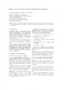
The use of such a process is motivated by statistical studies, which have shown that a model with constant Hurst index such as the fBm does not �t real life applications [6, 24]. Indeed fBm is a very rich model where a unique parameter, namely the Hurst index H , drives many properties: the correlation structure of the increments, the long range dependency, the self-similarity, and the roughness of the paths. Due to the time-varying Hurst index, stationarity of the increments does not hold anymore, therefore both long range dependency and structure of the increments are meaningless notions. For the mBm, only the roughness of the paths corresponds to the Hurst index H(t). However, this property is satis�ed under an extra-condition insuring that the Hölder regularity of the time-varying Hurst index t 7→ H(t) is greater than the maximum value of H(t), see e.g. [2, 6]. In order to allow very general probabilistic models, new generalisations of fBm or mBm have been introduced with a Hurst index which can be very irregular and even be itself a stochastic process, namely multifractional process with random exponent (MPRE) or generalised multifractional process (GMP) [2, 3]. Actually, we cannot know whether �uctuations re�ect reality or are just artefacts byproducts of statistics. This phenomenon is brought to light by the estimation of a time-varying Hurst index for a process X being a fBm with a constant Hurst index H = 0.7. Indeed Fig. 1 gives the 0.8 GQV Estimator Y Wavelet Estimator Y Linear Regression GQV Estimator Y (Fraclab) 0.78
0.76
0.74
0.72
0.7
0.68
0.66
0.64
0.62
0
0.5
1
1.5
2
2.5
3
3.5 4
x 10
b Figure 1: Estimation of a time-varying Hurst index H(t) for a fBm with constant Hurst index H = 0.7. feeling that the Hurst index is itself a stochastic process. In fact, the theoretical Hurst index is
P.R. Bertrand, M.E. Dury & N. Haouas
5
constant. But if we assume that this theoretical Hurst index is a time-varying function, namely
t 7→ H(t), then at each time t the Hurst index is estimated on a small vicinity around the time t. b Consequently, the sampling �uctuation induces that the time-varying estimator H(t) becomes a stochastic process. The same statistical artefact, providing the feeling that the estimated Hurst index behaves as a stochastic process, would occur for any time-varying Hurst index H(t) which is a C 1 function or a piecewise C 1 function. To sum up, the estimated Hurst index is a stochastic process, while the theoretical Hurst index is a deterministic function regularly varying with time. The same phenomenon appears in the article of Bardet-Surgailis [5, Fig. 2 and Fig. 3, pages 10231024]. Similarly, simulations presented in [13, Fig. 3, p.6] and [20, Fig. 1, p.1514] show a path of a mBm with a sine functional Hurst index H(t) with mean 1/2 and the corresponding time-varying b . Clearly, the theoretical Hurst index H(t) is a C ∞ function [20, Fig. 1 (c), Hurst index H(t)
b p.1514], whereas the estimated Hurst index H(t) looks like a continuous Hölder function with regularity α < 1, see [20, Fig. 1 (d), p.1514]. This remark led us to introduce a sparse mBm in [10] for application to �nancial processes. The guiding idea is to choose a simple function H(t) which describes the real dataset as well as a more complicated one. Let us stress that in this section, we have chosen to provide the underlying ideas, avoiding any technicality. 2
Recalls on fBM, mBm, and statistical estimation of Hurst index
2.1
Recalls on fBm and mBm
One of the most famous Gaussian random processes is the Brownian motion. At the beginning of the 20th century, this process was developed by Louis Bachelier for stock options in �nance and next by Albert Einstein in order to describe successive movements of atomic particules independent one from another. Then the mathematical theory is mainly due to Robert Wiener in the 1920's; he proved results on the non di�erentiability of the paths and the one-dimentional version is kwown as the Wiener process. The fractional Brownian motion (fBm) can hence appear as a generalisation of the Brownian motion. After the paper of Mandelbrot and Van Ness (1968), modeling by a fBm became more and more widespread, and the statistical study of fBm was developed during the decades 1970's and 1980's. Nevertheless, in many applications the real data do not perfectly �t with fBm. More precisely, statistical tests reject the null hypothesis H = 1/2 as it should be for Brownian motion or di�usion processes, but any alternative hypothesis would also be rejected when the Hurst index is varying with time. In fact, access to larger and larger datasets has shown that real time series look locally like
P.R. Bertrand, M.E. Dury & N. Haouas
6
a fBm, but with a time-varying Hurst index t 7→ H(t) rather than a constant one. This intuition was translated in mathematical modelling, by the introduction of multifractional Brownian motion (mBm) by Peltier, Lévy-Véhel (1995), and Benassi et al. (1997). Indeed, mBm is a continuous Gaussian process whose pointwise Hölder exponent evolves with time t. Recall that for the fBm, the pointwise Hölder exponent and Hurst index are equal. Therefore, a natural idea is to replace the Hurst index H by a function of time t 7→ H(t) in one of the representations of the fBm. Simultaneously, Peltier, Lévy-Véhel (1995) proposed to replace the Hurst index H by a time-varying one in the moving average representation, whereas Benassi et al.(1997) replaced it by a time-varying one in the harmonisable representation. Actually, both constructions correspond to the same process. Then, to be self-contained, we rely on the work of Ayache and Taqqu in [2] so we de�ne the multifractional Brownian motion (mBm) as follows:
De�nition 2.1 Let (t, H) 7−→ B(t, H) be the Gaussian �eld de�ned by (2). The multi-fractional
Brownian motion is de�ned by
(3)
X(t) = B(t, H(t)). 2.2
Estimation of the Hurst index for fBm and mBm
Let X be a fBm or a mBm. We observe one path of size n of the process X with mesh hn , � namely X(0), X(hn ), . . . , X(nhn ) . For simplicity and without real restriction, we can assume that hn = 1/n. We use quadratic variations to estimate the Hurst index. Let us �rst give the underlying idea: for a fBm with Hurst index H , we have
E |X (t + hn ) − X(t)|2
�
= |hn |2H .
(4)
On the one hand, the stationarity of the increments of fBm allows us to estimate the variance by the empirical variance and to get a central limit theorem (CLT). On the other hand, we can estimate the variance at M di�erent meshes of time, that is hn , 2hn , . . . , M hn ; then linear regression of the logarithm of the empirical variance at those di�erent meshes provides us an estimator of the Hurst index H . Moreover, a CLT is in force. Eventually, by a freezing argument, we can shift the technique from fBm to mBm. More precisely, let a = (a0 , . . . , a` ) be a �lter of order p, (tk )k=1,...,n a family of observation times, and X a fBm or a mBm. We de�ne the associated increment by
∆a X(tk ) =
` X
(5)
aq X(tk−q ).
q=0
Saying that a is a �lter of order p ≥ 1 means that ` X q=0
aq q k = 0 for all k < p
and
` X q=0
aq q p 6= 0.
(6)
P.R. Bertrand, M.E. Dury & N. Haouas
7
For example, a = (1, −1) is of order 1, whereas a = (1, −2, 1) is of order 2. Next, for a �lter (j)
(j)
a = (a0 , . . . , a` ) and any integer j ∈ N, we de�ne its j th dilatation a(j) = (a0 , . . . , aj` ) by (j)
(j)
aij = ai and ak = 0 if k ∈ / jN. Since X is a zero mean Gaussian process, ∆a(j) X(tk ) is also a zero mean Gaussian variable for any time tk and any dilatation j . For a fBm, that is when X = BH , its variance is 2H j Var [∆a(j) BH (tk )] = Ca × . n This variance can be estimated by the empirical variance. However, our aim is the estimation of the Hurst index for a mBm. The guiding idea is that a mBm behaves locally as a fBm. Therefore, we localise the estimation and we compute the empirical variance on a small vicinity of each time
t, namely on � V(t, εn ) = tk such that |tk − t| ≤ εn , where εn → 0 and εn /hn → ∞ as n → ∞. To sum up, given a �lter a and a real number
t ∈ (0, 1), we set Vn (t, a) =
1 vn
X
∆a X(tk ) 2
(7)
tk ∈V(t,εn )
where vn = 2εn /hn = 2εn × n is asymptotically equivalent to the number of times tk belonging to V(t, εn ). Eventually, we calculate the empirical variance at M di�erent scales j/n for j =
1, . . . , M . Then we set � At � (j) ln(V (t, a ) n 2AAt j=1,...,M
b n (t) = H
(8)
where A is the row vector de�ned by
Aj
= ln(j) −
M 1 X ln(ν) for j = 1, . . . , M M
(9)
ν=1
and At the transpose vector (column vector). Actually the number vn of terms in sum (7) converges to in�nity when n → ∞, thus a CLT is in force with a Gaussian limit. Then, the estimator of the Hurst parameter is also asymptotically Gaussian. More precisely, we can state the following proposition:
Proposition 2.1 (Coeurjolly, 2005�2006) Let a = (1, −2, 1) be a �lter of order 2 as de�ned
by (6), (tk = k/n)k=1,...,n a family of observation times, X = BH(t) a mBm with Hurst index a.s. b n (t) −→ H(t) and ∆a X the associate increments de�ned by (5). Then H H and n→∞
� √ b n (t) − H(t) 2εn · n × H �
D
−→ n→∞
G0 (t)
(10)
P.R. Bertrand, M.E. Dury & N. Haouas
8
where G0 (t) is a zero mean Gaussian process with covariance structure given by Var(G0 (t)) =
X 1 1 a πH(t) (k)2 a 2 4 2kAk πH(t) (0)
! × At (U U t )A
(11)
k∈Z
f or all t ∈ (0, 1), and
cov(G0 (t1 ), G0 (t2 )) = 0 f or all (t1 , t2 ) ∈ (0, 1)2 with t1 6= t2
(12)
where the row vector A is de�ned by (9) and U = (1, . . . , 1). Moreover, for a �lter a, and an integer k, the quantity πHa (k) is de�ned by `
`
1XX aq aq0 |q − q 0 + k|2H . 2 0
a πH (k) := −
(13)
q=0 q =0
To sum up, we set γH(t) := Var(G0 (t)) = ΛH (t) × (B.U.U t .B t )
with ΛH (t) =
X 2 a πH(t) (k)2 a πH(t) (0)2
(14)
k∈Z
and B =
At . 2kAk2
Proof. The proof can be obtained by combining [18, 19]. However, a more direct and natural proof is provided in Appendix A. 2
3
Statement of our main results
We propose a �tting test for a time-varying Hurst index and apply it to a model selection approach, leading to the simplest model. 3.1
Fitting test
As the selection of a good probabilistic model is the guideline of this article, the idea is now to give an adequacy test to select admissible estimators and reject others. For this, we use the
P.R. Bertrand, M.E. Dury & N. Haouas
9
previous convergence result. Actually, the CLT given in Proposition 2.1 leads to the following convergence in law:
√
� � b n (t) − H(t) 2εn · n × H
D
G0 (t)
−→ n→∞
for all t ∈ (0; 1) where (G0 (t), t ∈]0; 1[) is a zero mean Gaussian process which covariance structure is known. If H(.) is the theoretical index, then this means that we can explain the L2 risk b n (t) − H(t)k2 2 function, namely the MISE (Mean Integrated Squared Error) by EkH L (]0;1[) , where n
1X b |Hn (tk ) − H(tk )|2 n
b n (t) − H(t)k2 2 kH L (]0;1[) :=
k=1
with (tk =
k n )k=1,...,n
a family of observation times. Applying the previous CLT, we get the
convergence in law D
b n (t) − H(t)k2 2 2nεn kH L (]0;1[)
−→ n→∞
" n # 1 X 0 |G (tk )|2 . n
(15)
k=1
Set n
Vn :=
1X 0 |G (tk )|2 . n
(16)
k=1
We can deduce a CLT on Vn as stated in the following proposition
Proposition 3.1 Under the same assumptions than in Proposition 2.1. Let Vn be de�ned by
(16). We can rewrite Vn as follows
Vn = µn + Sn × ξn
(17)
with µn = E(Vn ) its mean, Sn = Var(Vn ) its standard deviation. Then we get the convergence in distribution to a standard normal deviate p
ξn
D
−→
N (0; 1).
n→∞
Proof. The proof is given in Appendix B. 2 As n converges to in�nity, we have
ˆ
1
E(Vn ) −→
γH(t) dt 0
and
�n� 2
ˆ × Var(Vn ) −→
1
(γH(t) )2 dt. 0
By replacing these quantities by their limits, we can formulate the �tting test:
(18)
P.R. Bertrand, M.E. Dury & N. Haouas
10
Theorem 3.1 Under the same assumptions as in Proposition 2.1 and Proposition 3.1, we can e test the eligibility of a function H(t) with the theoretical Hurst index. Namely set :
(19)
e (H0 ) : H(t) = H(t) e versus (H1 ) : H(t) 6= H(t). e Then H(t) is an eligible model if, for a given risk α, e |Tn (H(t))| ≤ uα e where Tn (H(t)) is de�ned by b n (t)) = Tn (H
2 b n (t) − H(t)k e 2nεn kH L2 (]0;1[) − � ´ �1/2 2 1 2 dt (γ ) e n 0 H(t)
´1 0
γH(t) e dt
(20)
!
where γH(t) := Var G0 (t) is given by Formula (11) and uα denotes the fractile of order (1 − α2 ) of the standard normal law. Proof. The proof is given in Appendix B. 2 e For instance, given a risk α = 0.05, we accept the null hypothesis if Tn (H(t)) ∈ [−1.96, 1.96]. 3.2
Application to model selection
b As a by-product, the naive time-varying estimator H(t) of the Hurst index could not be chosen e b as a valid model. Namely, it is not an admissible one. Nevertheless, the assumption H(t) = H(t) in the null hypothesis (19) is asymptotically rejected, as stated in the following corollary
e b n (t) we get Corollary 3.1 if H(t) =H
n
´1
r γH(t) e kL1 (]0;1[) e dt n kγH(t) = − × −→ ∞ as n → ∞ �1/2 2 kγH(t) e kL2 (]0;1[) 2 e ) dt 0 (γH(t)
− e Tn (H(t)) =� ´ 2 1
0
and then, as we are in the critical region, the null hypothesis (H0 ) is rejected. Proof. The proof is deduced from Theorem 3.1. 2 e The next idea is to determine the simplest possible function H(t) that will describe the theoretical Hurst index H(t). Note that such a model is in the same time simpler and �ts better the
P.R. Bertrand, M.E. Dury & N. Haouas
11
theoretical value of the Hurst index as it does not contain the statistical artefact. We are hence able to look for a suitable model; the aim is to determine the most simple model that is eligible for test (19). This model selection is a kind of Portemanteau test. Thus, for this, set
e M0 the family of constant models H(t) =H e M1 the family of a�ne models H(t) e M2 the family of piecewise a�ne models H(t) e M3 the family of quadratic models H(t) e . M4 the family of piecewise quadratic models H(t) We successively test models extracted from the previous families. Those families of models are e . We stop and use the �rst eligible model, classi�ed by order of complexity of function H(t) namely for family Mi with the lowest i. By construction of these families, the selected model is thus the simplest one. Conclusion
b n (t) is too complicated and has too many To sum up, the naive multifractional estimator H �uctuations that appear as a statistical artefact as shown in Fig. 1. Moreover, we have built a b n (t) as an appropriate estimator of the time-varying �tting test which asymptotically rejects H theoretical Hurst index H(t). Next, this �tting test is used to select the simplest time-varying e Hurst index H(t) from a given families of models, by a Portemanteau procedure. We have proposed in Sect. 3.2 a family of piecewise polynomial functions. However di�erent choices are possible such as logistic functions, see e.g. [25, Fig. 2, p.101]. In a certain way, our work con�rms and enhances the multifractional process with random Hurst exponent (MPRE) introduced by Ayache and Taqqu (2005) [2]. Indeed, the Hurst exponent could be random without being itself a stochastic process. For instance a piecewise a�ne (or quadratic function) with change of slope at random times is still a random exponent, without having to oscillate roughly, see e.g. [10, Fig. 6, p. 15]. So, we have disentangled a random timevarying Hurst exponent from a roughly oscillating exponent resulting from a statistical artefact. This result also better �ts the interpretations proposed by scholars from applied �elds: it is simpler to interpret a slowly varying function taking values larger or smaller than the nominal value [30, 25, 35, 14, 20]. Let us add that the selected model is both simpler and �ts better the theoretical value of the Hurst index H(t). Consequently, this study opens the way to further research like online detection of change of slope of the Hurst index or study of the di�erent kinds of families of model.
P.R. Bertrand, M.E. Dury & N. Haouas
12
References
[1] Ayache, A, Bertrand, PR, Lévy-Véhel J (2007), A Central Limit Theorem for the Generalized Quadratic Variation of the Step Fractional Brownian Motion.
Stochastic Processes 10, 1�27.
Statistical Inference for
[2] Ayache, A, Taqqu, MS (2005), Multifractional processes with random exponent.
Publ. Mat.
49, 459�486. [3] Ayache, A, Ja�ard, S, Taqqu, MS (2007) Wavelet construction of Generalized Multifractional processes.
Revista Matematica Iberoamericana, 23, No 1, 327�370.
[4] Bardet, JM, Bertrand, PR (2007). De�nition, properties and wavelet analysis of multiscale fractional Brownian motion.
Fractals 15, 73�87.
[5] Bardet, JM, Surgailis, D (2013). Nonparametric estimation of the local Hurst function of
Stochastic Processes and Applications, 123, 1004�1045. [6] Benassi A, Ja�ard S, Roux D (1997), Elliptic Gaussian random processes. Revista Matematica Iberoamericana, 13(1):19-90. multifractional processes.
[7] Benassi A, Bertrand PR, Cohen S, Istas J (2001) Identi�cation of the Hurst index of a step fractional Brownian motion.
Statistical Inference for Stochastic Processes 3( 1/2): 101�111.
[8] Bertrand, PR, Bardet, JM (2001) " Some generalization of fractional Brownian motion and Control", in
Optimal Control and Partial Di�erential Equations, J.L. Menaldi, E. Rofman
and A. Sulem editors, p.221-230, IOS Press. [9] Bertrand, PR (2005) "Financial Modelling by Multiscale Fractional Brownian Motion.", in
Fractals in Engineering. New trends in theory and applications, edited by Lutton E. and Levy Vehel J., p.159-175, Springer Verlag. [10] Bertrand, PR, Hamdouni, A, Khadhraoui S (2012), Modelling NASDAQ series by sparse multifractional Brownian motion,
Methodology and Computing in Applied Probability. Vol.
14, No 1: 107�124. [11] Bianchi, S (2005) Pathwise Identi�cation of the memory function of multifractional Brownian motion with application to �nance.
Finance Vol. 8, No. 2, 255�281.
International Journal of Theoretical and Applied
[12] Bianchi, S, Pianese, A (2008) Modeling Stock Prices by Multifractional Brownian Motion: An Improved Estimation of the Pointwise Regularity
and Applied Finance Vol.11, No 6, 567�595.
International Journal of Theoretical
[13] Bianchi, S, Pantanella, A, Pianese, A (2011) Modeling Stock Prices by Multifractional Brownian Motion: An Improved Estimation of the Pointwise Regularity 13(8)
Quantitative Finance
P.R. Bertrand, M.E. Dury & N. Haouas
13
[14] Bianchi, S, Pantanella, A, Pianese, A (2015) E�cient Markets and Behavioral Finance: a comprehensive multifractal model.
Advances in Complex Systems 18.
[15] Bianchi, S, Pianese, A (2014) Multifractional Processes in Finance. SSRN Electronic Journal 5(1):1-22 [16] Breuer, P, Major, P (1983) Central Limit Theorems for Non-Linear Functionals of Gaussian Fields.
J.of Multivariate Analysis 13, 425�441.
[17] Cheridito P(2003) Arbitrage in Fractional Brownian Motion Models.
Finance Stoch. 7(4):
533�553. [18] Coeurjolly, JF (2005), Identi�cation of multifractional Brownian motion,
Bernoulli 11 (6),
987�1008. [19] Coeurjolly, JF (2006), Erratum:
Identi�cation of Multifractional Brownian Motion,
Bernoulli 12 (2), 381�382. [20] Frezza, M (2012) Modeling the time-changing dependence in stock markets.
& Fractals 45(12):1510�1520
Chaos Solitons
[21] Guyon, X, Leon, JR (1989), Convergence en loi des H-variations d'un processus gaussien fractionnaire.
Ann. Inst. H. Poincaré 25 (3), 265�282.
[22] Istas, J, Lang, G (1997), Quadratic variation and estimation of the local Hölder index of a Gaussian process.
Ann. Inst. H. Poincaré 33 (4), 407�437.
[23] Kolmogorov AN (1940) Wienersche Spiralen und einige andere interessante Kurven in Hilbertchen Raume. Doklady 26: 115�118. [24] Peltier, RF, Lévy-Véhel, J (1995), Multifractional Brownian motion: de�nition and preliminary results, Research Report RR-2645, INRIA, Rocquencourt, http://www.inria.fr/rrrt/rr2645. html. [25] Lee KC (2013) Characterization of turbulence stability through the identi�cation of multi-
Nonlinear Processes in Geophysics 20(1):97-106. [26] Mandlebrot, BB (2012) The fractalist. Memoir of a Scienti�c Maverick. Pantheon. fractional Brownian motions
[27] Lim SC , Teo LP (2009) Modeling Single-File Di�usion by Step Fractional Brownian Motion and Generalized Fractional Langevin Equation. Journal of Statistical Mechanics Theory and
Experiment
[28] Marquez-Lago TT, Leier A, Burrage K. Anomalous di�usion and multifractional Brownian motion: simulating molecular crowding and physical obstacles in systems biology
Systems Biology 6(4):134-42.
IET
[29] Ryvkina, J (2013), Fractional Brownian Motion with variable Hurst parameter: De�nition and properties. Journal of Theoretical Probability DOI 10.1007/s10959-013-0502-3 Print ISSN 0894-9840
P.R. Bertrand, M.E. Dury & N. Haouas
14
[30] Papanicolaou, G, Sølna, K (2002) Wavelet based estimation of local Kolmogorov turbulence. In: P. Doukhan, G. Oppenheim and M.S. Taqqu (eds), Long-range
Dependence: Theory and
Applications, Birkhäuser, Basel, (2002), 473-506.
[31] Rásonyi M (2009) Rehabilitating Fractal Models in Finance.
ERCIM News: 19�20.
[32] Rogers LCG (1997) Arbitrage with fractional Brownian motion.
Mathematical Finance 7:
95�105. [33] Samorodnitsky, G, Taqqu MS (1994),
Stable non-Gaussian Random Processes, Chapman
and Hall. [34] Shiryaev AN (1998) On arbitrage and replication for fractal models. Technical report. MaPhySto. [35] Wanliss JA, Dobias, P (2007) Space storm as a phase transition
and Solar-Terrestrial Physics 69 (2007) 675-684. A
Journal of Atmospheric
Proof of Proposition 2.1
The proof is divided in three steps. Both Step 1 and Step 2 are concerned with fBm. In Step 1, we prove a CLT for the localised quadratic variations of order 2 of the fBm. In Step 2, we deduce a CLT for the estimator of Hurst index obtained by linear regression of the logarithm of quadratic variation at di�erent meshes of times for fBm. Next, Step 3 explains how to shift from fBm to mBm. Before going further, let us state a technical lemma used in Step 1.
Lemma A.1 Let a be a �lter of order p ≥ 1 as de�ned by (6), (tk = k/n)k=1,...,n a family
of observation times, X = BH a fBm with covariance given by (1), and ∆a X the associate increments de�ned by (5). Then 1. ∆a X(.) is a zero mean Gaussian vector, with covariance structure given by cov [∆a X(tk ), ∆a X(tk0 )] = σ2 n−2H πHa (k − k0 )
(21)
for all pair (k, k0 ), where πHa (k) is de�ned by (13). 2. As a by-product, for all k Var [∆a X(tk )] = E ∆a X(tk ) 2 = σ2 n−2H πHa (0).
(22)
3. Moreover, for all k ∈ Z a πH (k) ≤ Ctte × |k|2H−2p .
(23)
P.R. Bertrand, M.E. Dury & N. Haouas
15
Remark A.1 Formula (22) implies that Var [∆a X(tk )] = Ctte × h2H n , with hn = 1/n. This
proves and generalises formula (4).
Proof. 1) and 2) Since X = BH is a zero mean Gaussian process, we deduce that ∆a X(tk ) is a zero mean Gaussian vector, with covariance structure given by cov [∆a X(tk ), ∆a X(tk0 )] =
` X ` X
� � aq aq0 cov BH (tk−q ), BH (tk0 −q0 )
q=0 q 0 =0
=
` ` � σ2 X X aq aq0 |tk−q |2H + |tk0 −q0 |2H − |tk−q − tk0 −q0 |2H 2 0 q=0 q =0
` ` σ2 X X aq aq0 |tk−q − tk0 −q0 |2H , = − 2 0 q=0 q =0
where the last equality follows from Eq.(6). Next, by setting tk = k/n, we can deduce Formula (21). As pointed in Lemma A.1, Formula (22) follows from Formula (21). 3) See Coeurjolly (2001, lemma 1). 2
Step 1: CLT for quadratic variations of fBm. For a fBm X = BH , the variance of the increments does not depend on the time tk , see Lemma A.1 Formula (22). Thus from (7) we get # " 2 X ∆a X(tk ) 1 Vn (t, a) = Var [∆a X(tk )] × 1 + 2 − 1 vn tk ∈V(t,εn )) E ∆a X(tk ) ( ) � �2H 1 2 a = σ πH (0) × 1 + Ven (t, a) n
(24)
where
Ven (t, a) :=
1 vn
X
��
� (a) 2
Zk
� −1
tk ∈V(t,εn ))
and (a)
Zk
∆a X(tk ) := q 2 . E ∆a X(tk )
(25)
For notational convenience, we drop the index (a) in the sequel, and we note that for k = 1, . . . , n,
Zk forms a stationary family of zero mean standard Gaussian variables with correlation r(k) = corr(Zj , Zj+k ) =
a (k) πH a (0) πH
(26)
P.R. Bertrand, M.E. Dury & N. Haouas
16
a is de�ned by (13). Actually, Z 2 − 1 = H (Z ) where H (x) = x2 − 1 is the Hermite where πH 2 2 k k
polynomial of order 2. By using Breuer-Major Theorem [16], a CLT with a Gaussian limit is in X force as soon as r(k)2 < ∞. Combining Formula (26) and Bound (23) in Lemma A.1, we k∈Z 2
deduce that r(k) = O(k 4H−4p ). The series
X
k 4H−4p converges if and only if 4H − 4p < −1
k∈Z
or equivalently i� H < p − 1/4. So, for p = 1 which corresponds to the case a = (1, −1) and quadratic variations, we get a CLT i� H < 3/4; whereas for p = 2 with a = (1, −2, 1), and the socalled generalised quadratic variations (GQV), the CLT is in force for all Hurst index H ∈ (0, 1). For these reasons we do prefer the use of GQV rather than simple quadratic variations, see also Istas-Lang or Guyon-Leon. a (0) = 4 − 22H . Note that for a = (1, −2, 1), we get πH √ √ The rate of convergence is vn = 2nεn . Moreover,
� � h �i 2 E H2 (Zk ) · H2 (Zk0 ) = 2 E Zk · Zk0 . This relation combined with (26) involves the following calculation of the variance n�√ X X �2 o 1 vn · Ven (t, a) = E × E(H2 (Zk ) · H2 (Zk0 )) vn 0 k,tk ∈V(t,εn ) k ,tk0 ∈V(t,εn ) h i2 X X 2 E(Zk · Zk0 ) × = vn 0 k,tk ∈V(t,εn ) k ,tk0 ∈V(t,εn )
= =
� π a (k)2 vn − |k| × H a (0)2 πH |k| 0, we have X(t) − BH(t ) (t) ≤ C1 (ω) × εη , 0
f or all t ∈ V(t0 , ε).
P.R. Bertrand, M.E. Dury & N. Haouas
19
Proof. Indeed, from Th. A.1 and Hölder continuity, we get: X(t) − BH(t ) (t) ≤ C2 (ω) × |H(t) − H(t0 )| 0 ≤ C2 (ω) × M1 |t − t0 |η ≤ M1 · C2 (ω) × εη , for all t such that |t − t0 | ≤ ε. By setting C1 (ω) = M1 · C2 (ω), this �nishes the proof of Cor. A.1.
2 From Cor. A.1, we then get (31)
X(t) = BH0 (t) + ξ(t) for all t ∈ V(t0 , εn ) =]t0 − εn , t0 + εn [, where H0 = H(t0 ), η is the Holder regularity of map t 7→ H(t), for t in the vicinity of t0 ,
and | ξ(t)| ≤ C1 (ω) εηn where the random variable C1 has �nite moment of every order. We deduce from (31) that
∆a X(t) = ∆a BH0 (t) + ∆a ξ(t), for all t ∈ V(t0 , εn ) =]t0 − εn , t0 + εn [. Our strategy, in the rest of the proof of Step 3, is to make an expansion in the vicinity of time t0 , then around BH0 . Indeed, since εn = n−α , for all
t ∈ V(t0 , ε), we have ∆a BH0 (t) ∼ n−H0
and
∆a ξ(t) ≤ 2 C1 (ω) n−αη .
(32)
The condition (33)
α · η > H0
insures that ∆a ξ(t) is in�nitely smaller than ∆a BH0 (t), uniformly for all t ∈ V(t0 , ε). Then Vn , as de�ned by (7), becomes
Vn (X, t0 , a(j) ) =
1 vn
X
n o ∆a BH (tk ) 2 + 2∆a BH (tk ) · ∆a ξ(tk ) + ∆a ξ(tk ) 2 0 0
tk ∈V(t0 ,εn )
2 = Vn (BH0 , t0 , a(j) ) + vn
X tk ∈V(t0 ,εn )
∆a BH0 (tk ) · ∆a ξ(tk ) + Vn (ξ, t0 , a(j) )
P.R. Bertrand, M.E. Dury & N. Haouas
20
We can easily deduce from (32) and condition (33), that X 2 ∆a BH0 (tk ) · ∆a ξ(tk ) + Vn (ξ, t0 , a(j) ) vn tk ∈V(t0 ,εn )
is in�nitely smaller than Vn (BH0 , t0 , a(j) ). Next Taylor expansion induces � P � 2 ∆ B (t ) · ∆ ξ(t ) + Vn (ξ, t0 , a(j) ) a a H k k 0 t ∈V(t ,ε ) vn 0 n k ln Vn (X, t, a(j) ) = ln Vn (BH0 , t, a(j) ) + Vn (BH0 , t0 , a(j) ) By Cauchy-Schwarz inequality, we get 1 X ∆a BH0 (tk ) · ∆a ξ(tk )Vn (BH0 , t0 , a(j) ) ≤ Vn (BH0 , t, a(j) )1/2 × Vn (ξ, t0 , a(j) )1/2 vn tk ∈V(t0 ,εn )
which implies
ln Vn (X, t, a(j) ) = ln Vn (BH0 , t0 , a(j) ) + 2µ θn1/2 + θn where µ ∈ [−1, 1] and θn =
(34)
Vn (ξ, t0 , a(j) ) . Vn (BH0 , t, a(j) )
Lemma A.2 Under the same assumptions as previously, 0 θn ≤ C3 (ω) × ε2η n
(35)
where the variable C3 has �nite moment of every order and η0 = η − Hα0 . Proof. Cor. A.1 implies the bound (32), which induces Vn (ξ, t0 , a(j) ) ≤ 2 C1 (ω) n−2αη . Indeed, 2 Vn (ξ, t0 , a(j) ) is the average of the quantities ∆a ξ(tk ) for tk ∈ V(t0 , εn ), which are uniformly bounded by 2 C1 (ω) n−2αη . Next, by using formula (27) we get
θn ≤
2 C1 (ω) j 2H0 n o × n−2(αη−2H0 ) a σ 2 π (0) × 1 + Ven (t0 , a(j) ) H
≤
2 j 2H0 C1 (ω) 0 n o × ε2η n a (0) × σ 2 πH (j) 1 + Ven (t0 , a )
This proves the bound (35) with
C3 (ω) =
2 j 2H0 C1 (ω) o. ×n a 2 σ πH (0) 1 + Ven (t0 , a(j) )
P.R. Bertrand, M.E. Dury & N. Haouas
21
Then, it remains to prove that C3 has �nite moments, namely that
1 E n ol < ∞, 1 + Ven (t0 , a(j) ) for all l ∈ N. For this, by Hölder inequality, we get
�
∀l ∈ N, E |C3 (ω)|l where
1 p
+
1 q
�
�1 q ≤ E C1lq (ω) × E
1
�
!1
p
(1 + Ven (t0 , a(j) ))lp
= 1. We deduce from Corollary A.1 that � � E C1lq (ω) < +∞.
Thus it remains to prove that the other part as �nite moments of any order : ! 1 E < +∞. (1 + Ven (t0 , a(j) ))lp But from Formula (24) (see Step 1) we get (j)
1 + Ven (t0 , a
1 )= vn
X tk ∈V(t,εn ))
" # ∆a BH (tk ) 2 0 � Var ∆a BH0
where ∆a BH0 (tk ) is a centered Gaussian random variable. Therefore we get
1 1 + Ven (t0 , a(j) ) = vn
X
2 Zk
tk ∈V(t,εn ))
∆BH0 (tk ) where Zk is a standard random variable de�ned by (25) as Zk := q . Moreover Var ∆BH0 (tk ) D random variables Zk are weakly dependent, which implies that 1 + Ven (t0 , a(j) ) −→ χ2dn , see e.g. n→∞
Istas-Lang 1997 [22] or Ayache-Bertrand-Lévy-Vehel 2007 [1], with dn → +∞ as n → +∞. We can deduce that
1 E
(1 + Ven (t0 , a(j) ))lp
! ' E ˆ
1 (χ2dn )lp ∞
= ˆ0 ∞ = This �nishes the proof of Lemma A.2. 2
1 dn −1 −t/2 t2 e dt tlp t
0
!
dn −lp−1 2
e−t/2 dt < ∞.
P.R. Bertrand, M.E. Dury & N. Haouas
22
Next using (29) combined with (34) and Lemma A.2, we get
� At � (j) ln V (X, t , a ) n 0 2AAt j=1,...,M � At � (j) 1/2 , t , a ) + 2µ θ + θ = ln V (B n n H0 0 n 2AAt j=1,...,M 0 η b = Hn (BH0 , t) + O(εn ).
b n (X, t) = H
But for each �xed Hurst index H0 , the following CLT, given by (10), holds � � √ D b n (BH , t0 ) − H0 −→ G0 (t). 2εn · n × H 0 n→∞
This CLT remains in force for mBm X as soon as the freezing error is negligible with respect to the rate of convergence of the estimator of the Hurst index for fBm, namely 0
εηn �
√
2εn · n.
By taking εn = n−α we get the following condition p 0 n−α εηn � 2n × n−α namely 0
n−α εηn �
√
2n
α−1 2
which means that the Necessary and Su�cient Condition is
2αη 0 > 1 − α which is equivalent to
α>
1 := φ(η 0 ). 1 + 2η 0
This �nishes the proof of Step 3 (freezing) and consequently the proof of Proposition 2.1. B
Proof of our main result - Theorem
3.1
Using CLT given in Proposition (2.1), by Formula (10) we get this convergence in law: � � √ D b n (t) − H(t) 2εn · n × H −→ G0 (t) n→∞
for all t ∈ (0; 1) where (G0 (t), t ∈]0; 1[) is a zero mean Gaussian process which covariance structure is known. If H(.) is the real index, then this means that we can explain the L2 risk function, b n (t) − H(t)k2 2 namely the MISE (Mean Integrated Squared Error) by EkH L (]0;1[) , where n
1X b b n (t) − H(t)k2 2 kH |Hn (tk ) − H(tk )|2 L (]0;1[) := n k=1
P.R. Bertrand, M.E. Dury & N. Haouas
23
with (tk = nk )k=1,...,n a family of observation times. Applying the previous CLT, we get (15): " n # X 1 D b n (t) − H(t)k2 2 −→ 2nεn kH |G0 (tk )|2 . L (]0;1[) n n→∞ k=1
We can hence use it under the following form
b n (t) − kH
H(t)k2L2 (]0;1[)
'CT L
" n # 1X 0 1 2 |G (tk )| . 2nεn n k=1
Set Vn de�ned by (16)
n
Vn :=
1X 0 |G (tk )|2 . n k=1
We here aim at proving that Vn satis�es a CTL.
Proof. Up to a multiplicative factor, it su�cies to prove the CLT for Ven de�ned by Ven := n × Vn =
n X
|G0 (tk )|2 .
k=1
For this, we can apply the CLT proved in [1, Th 3.1]
Ven = µ en + Sen × ξn and consequently Formula (17)
Vn = µn + Sn × ξn where µn = E(Vn ) is the expected value, Sn =
p Var(Vn ) is the standard deviation, and the
following convergence in distribution to a standard normal deviate (18) holds
ξn
D
−→
N (0; 1).
n→∞
Actually, as G0 (tk ) are Gaussian centred random variables, we can apply a result from Istas-Lang (2007) [22]. A su�cient condition to get result (18) is " !# Pn 0 0 maxk∈{1,...,n} j=1 cov G (tk ); G (tj )
lim
n−→∞
= 0.
q Var(Ven )
(36)
For j 6= k , if tj and tk where adequately located, namely at a su�cient distance each other (N , with N −→ ∞), we would have
! cov G0 (tk ); G0 (tj )
= 0.
(37)
P.R. Bertrand, M.E. Dury & N. Haouas
24
Then, as G0 (tk ) are Gaussian random variables with zero mean, we just keep ! ! ! n X cov G0 (tk ); G0 (tj ) = Var G0 (tk ) = E G0 (tk )2 . j=1
Next, it comes that
" max k∈{1,...,n}
n X
!# 0
0
cov G (tk ); G (tj )
" =
max k∈{1,...,n}
j=1
!# 0
Var G (tk )
.
! From Proposition (2.1), formula (11) gives us the expression of Var G0 (tk )
! Var G0 (tk )
= γH(tk ) .
On the other hand, by de�nition of Ven and by assumption (37) of independence of Gaussian random variables G0 (tk ), we can write that Var(Ven ) =
n X
! Var G0 (tk )2 .
(38)
k=1
As G0 (tk ) is Gaussian, the variance of G0 (tk )2 can be explained in the following way
! 0
Var G (tk )
2
!2 #
" 0
0
2
2
G (tk ) − E(G (tk ) )
= E "
#
= E G0 (tk )4 − (E[G0 (tk )2 ])2 #2
" 0
= 2 × Var(G (tk )) and it comes that
!2
! Var G0 (tk )2
=2×
γH(tk )
.
Then su�cient condition (36) becomes
! maxk∈{1,...,n} lim v u uPn t
γH(tk ) ! =0
n−→∞
k=1
2 × (γH(tk ) )2
(39)
P.R. Bertrand, M.E. Dury & N. Haouas
25
since
!
! maxk∈{1,...,n} v u uPn t
k=1
γH(tk )
2 × (γH(tk
maxk∈{1,...,n}
!≤v u u t2n × min 2 ))
γH(tk ) !2 #
"
k∈{1,...,n}
γH(tk )
so this condition is satis�ed and CLT (Th.3.1 in [1]) holds. We hence have proved that CLT (17) holds. Then, by de�nition of Vn , we have ! ! n n n X 1 1X 1X Var G0 (tk ) = E G0 (tk )2 = γH(tk ) E(Vn ) = n n n k=1
k=1
(40)
k=1
and
# " n X 2 1 1 2 (γH(tk ) ) Var(Vn ) = 2 Var(Ven ) = n n n
(41)
k=1
ˆ
1
using respectively (38) and (39). From (40) we get that E(Vn ) −→ γH(t) dt, and from (41), 0 ˆ �n� 1 we get that × Var(Vn ) −→ (γH(t) )2 dt as n → ∞. Consequently, set as in Formula (20): 2 0
b n (t)) = Tn (H
b n (t) − H(t)k2 2 2nεn kH L (]0;1[) − � ´ �1/2 2 1 2 dt (γ ) H(t) n 0 D
´1 0
γH(t) dt
Combining (15) and (18) we get that Tn −→ N (0, 1) as n → ∞. 2 n→∞
.