Selective Smoothing of the Generative Topographic ...
Recommend Documents
pipeline carrying a mixture of oil, water and gas (Bishop and James 1993). Each data ..... We would like to thank Geoffrey Hinton, Iain Strachan and Michael.
It also provides a principled alternative to the self-organizing map | a widely estab
- lished neural ...... on Arti cial Neural Networks, Cambridge, 1997, chapter 4,.
(Tréguier et al. 1999) showed only few differences in the LEVEL solution when using 72 levels instead of. 43. The previous vertical resolution in SIGMA (20 lev-.
use in extending the GTM to tree-structured data is presented in Section V. We ...... a cartesian coordinate system {e1, e2} in V. Its area is equal to dA = dx1dx2.
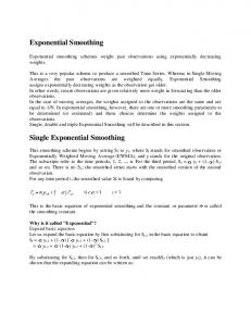
a rule based grammar. ...... level of magnification; brighter squares are associated with ... too, clearly separated by bright boundaries signifying stretches.
of neural network that allows a nonlinear projection of data residing in a high ... The Generative Topographic Map (GTM) algorithm [4] was introduced as a ...... for adaptive processing of structured data,â Neural Networks, IEEE. Transactions on ..
(GTM) for data visualization, structure-activity modeling and database comparison is evaluated, on hand of subsets of the Database of Useful Decoys (DUD).
analyzing a large data set on the customers, the structure of data can be highly ... methods in analyzing the web customer data and compared their rela-.
Keywords: Image Processing; Speckle Noise Smoothing; Selective Filter; Medical imaging; Female .... Noise removal is a common task in digital image processing and it has been widely studied. This ..... smoothing to be varied by modifying the size of
Feb 2, 2018 - Let V be the value function of the mini-minimax game defined as min. {gk} min .... [4] Phillip Isola, Jun-Yan Zhu, Tinghui Zhou, and Alexei A. Efros, ... [9] Jost Tobias Springenberg, âUnsupervised and Semi-supervised. Learning ...
In addition, data from experiments with nine monkeys previously de- scribed by Insausti et al. ... 20% glycerol solutions in 0.1 M phosphate buffer of pH 7.4. All brains were sectioned at 30 .... layer III by a cell-free zone. Area 36 is located just
on both the quality of the electroencephalogram (EEG) recording and the expertise of .... standard deviation of 20 s of noise-free background EEG selected as reference ..... Misulis KE. Spehlmann's evoked potential primer: Visual, auditory and ...
Exponential smoothing schemes weight past observations using exponentially ...
equal to 1/N. In exponential smoothing, however, there are one or more ...
and the best modulation frequency (BMF) were measured using AM signals (modulation fre- quencies up to 5 kHz and carrier frequency either equal or much ...
Examining the nature of control in generative art could reveal different viewpoints ..... [11] G. Flake, The Computational Beauty of Nature, The MIT Press, 1998.
In [yelp], 31 must be analyzed as an initial consonant, since y does not form a rising diph- thong with the head sonant e. In liyedf, on the other hand, y must be.
Examining the nature of control in generative art could reveal different viewpoints ..... [11] G. Flake, The Computational Beauty of Nature, The MIT Press, 1998.
Mar 29, 2013 - We give an application to counting subdiagrams of pretzel knots which have one component after oriented and unoriented smoothings. 1.
May 21, 1999 - are all based on a Gaussian-like convolution followed by an analysis of ..... Recall the de nitions of erosion and dilation of a subset X ...... 34] B. Julesz, Texton gradients: the texton theory revisited, Biological Cybernetics, 54,
has been the growth of the personal computer (PC): an affordable, multifunctional device ..... other), a piece of paper (hosting written language), or an alphabet ..... dedicated word processing appliances^^ have been trounced by PCs running ...
Thirdly, and related to the point above, the lexicon is not just verbs. Recent work ..... (Montague 1974). But we will see that ..... Romeo gave the lecture. b.Hamlet ...
British Army's Ro Allen Company at Sandhurst in the 1950's (Adair, 1998). .... from the business perspective, treating the experience as product and packaging it for ..... Dubuque,. Iowa. Wurdinger, S. (1994). Philosophical Issues in Adventure ...
Mar 16, 2017 - Threedimensional view of Bingham Canyon Mine, Utah, a humanmade topographic signature, based on a free, openaccess highresolution ...
M. Rezo, D. MarkovinoviÄ, M. Å ljivariÄ. Utjecaj Zemljinih ... deflection, we distinguish the following methods: ... Influence of the Earth's topographic masses on vertical deflection. M. Rezo, D. ... The astro-geodetic method of determining the va
Selective Smoothing of the Generative Topographic ...
5. Gray-scale map representing the magnitude of the regularization parameters , from SMS of surface B. Light shades of gray correspond to high values of and, ...
IEEE TRANSACTIONS ON NEURAL NETWORKS, VOL. 14, NO. 4, JULY 2003
1
Selective Smoothing of the Generative Topographic Mapping A. Vellido, W. El-Deredy, and P. J. G. Lisboa
Index Terms—Automatic relevance determination (ARD), Bayesian probability theory, generative topographic mapping (GTM), regularization, self-organizing map (SOM).
I. INTRODUCTION
T
in the data space back to produce a posteriori probability of each point in latent space. GTM uses a well-defined objective function whose optimization, using either standard techniques for nonlinear optimization or the expectation–maximization (EM) algorithm, has been shown to converge. Training GTM using the Bayesian approach allows for the automatic calculation of the model’s learning parameters, including a hyperparameter for regularization [2]. In this paper, we extend the automatic relevance determination (ARD) formulation to GTM. Multiple regularization parameters—one associated with each of the basis functions—are introduced to selectively and locally control the smoothness and over-parameterization of the mapping from the latent space to the data space, according to the inhomogeneities of the data. The regularization coefficients control the contribution of each basis function to the mapping and, hence, optimize the effective number of basis functions, in a manner analogous to the soft-pruning of irrelevant input variables with ARD [3].
IE E Pr E oo f
Abstract—Generative topographic mapping is a nonlinear latent variable model introduced by Bishop et al. as a probabilistic reformulation of self-organizing maps. The complexity of this model is mostly determined by the number and form of basis functions generating the nonlinear mapping from latent space to data space, but it can be further controlled by adding a regularization term to increase the stiffness of the mapping and avoid data over-fitting. In this paper, we improve the map smoothing by introducing multiple regularization terms, one associated with each of the basis functions. A similar technique to that of automatic relevance determination, our selective map smoothing locally controls the stiffness of the mapping depending on length scales of the underlying manifold, while optimizing the effective number of active basis functions.
HE lack of a unified statistical framework for the treatment of learning in neural networks has often been adduced as a limitation of these models. One such framework, based on Bayesian probability theory, was proposed and developed by MacKay [4] for the multilayer perceptron (MLP) The application of the Bayesian approach to the training of neural networks has important modeling implications, namely it requires modeling assumptions, including the specification of prior distributions, to be made explicit; as a modeling framework, it automatically satisfies the likelihood principle; it also provides a natural framework to handle uncertainty [3]. The Bayesian approach has other useful features, such as the automatic calculation of hyperparameters, including estimations of data noise and the regularization coefficients. The generative topographic mapping (GTM) is a latent variable model introduced by Bishop et al. [1] as probabilistic formulation of the well-known self-organizing map (SOM) [5]. GTM is a nonlinear (topographically preserving) mapping from a low-dimensional latent space [usually one- or two-dimensional (1-D) or (2-D)] onto the multidimensional data space. The mapping is carried through by an intermediate set of basis functions generating a (mixture) density distribution in the data space. Bayesian theory can be used to map points
Manuscript received May 9, 2001; revised June 5, 2002 and February 26, 2003. The authors are with the School of Computing and Mathematical Sciences, Liverpool John Moores University, Liverpool L3 3AF, U.K. (e-mail: [email protected]). Digital Object Identifier 10.1109/TNN.2003.813834
II. GTM AND THE EVIDENCE FRAMEWORK
GTM describes a nonlinear low-dimensionality latent variable model that generates a probability density in the multidimensional data space through a linear mixture of basis functions (1)
where is a point in data space, is an -dimensional point is the matrix that generates the explicit mapin latent space, ping from latent space to an -dimensional manifold embedded in data space, and is a set of basis functions which, in this paper, are chosen to be Gaussians. In order for the nonlinear mapping to remain analytically and computationally tractable, , in latent space is usually conthe prior distribution of , strained to a sum of delta functions, forming a uniform discrete grid, analogous to the distribution of nodes in the SOM (2)
is a pre-set number of nodes determining the grid size where or resolution. Since the data do not necessarily lie in a smooth -dimensional manifold, it is necessary to define a noise model for the distribution of the data points . The log-likelihood of fitting the data from the latent variables is given by
IEEE TRANSACTIONS ON NEURAL NETWORKS, VOL. 14, NO. 4, JULY 2003
which is empirically estimated by summing over the input data . Parameters, and , can be determined using the set EM algorithm [6], details of which can be found in [1]. The smoothness of the mapping generated by the GTM model is mainly determined by the number and form of the basis functions. Further model complexity control can be achieved with the addition of a regularization term to the error function (3), in such a way that the training of the GTM would consist of the maximization of a penalized log-likelihood
where all the constant terms have been grouped as . The maximization of this expression for and leads to the standard updating formulae of the evidence approximation (11) where (12)
(4)
(13)
where , , and have all been previously defined, is the responsibility or posterior probability of each GTM node for is the result of mapping each data point [1], and the discrete node representation into data space (2). In practice, the updating of the hyperparameters is intertwined with the calculations of the EM algorithm. The advantage of the evaluation of the complexity parameters within this framework is that, instead of having to resort to the calculation of the determinant of Hessians, only the derivative of the evidence with respect to the hyperparameters is required. The latter makes use of the trace of the inverse of the Hessian, which is numerically better conditioned [3].
IE E Pr E oo f
where is a regularization coefficient, and is a vector shaped by concatenation of the different column vectors of the weight matrix . This regularization term is important to prevent the GTM from fitting the noise in the data. Given that the GTM is formulated within a probabilistic framework, the optimization of its complexity-controlling parameters can be accomplished using the Bayesian formalism and, more specifically, the evidence approximation [4]. Since and control other parameter distributions, they are referred to as hyperparameters. The application of this methodology to and , as developed in [2], is summarized next. The best point estimates of the values of the hyperparameters are the mode of the posterior distribution
. and are the eigenvalues of The estimate of the inverse variance of the noise model, , now becomes
(5)
If uninformative priors are chosen, this is equivalent to maximizing the evidence or marginal likelihood
(6)
III. SELECTIVE MAPPING SMOOTHING (SMS)
(7)
The calculation of the optimum number of effective basis functions can also be accomplished within the Bayesian framework. Here, we propose using the method of ARD [3] for that purpose. Instead of using a single regularization coefficient for the whole mapping, a different regularization coefficient is defined for each basis function. In this way, the prior distribution over the weights (7) becomes
The usual normal prior is chosen for the weights
where is the number of weights in ). Let us now define
(with dimensions
(8)
Using a second-order Taylor expansion of (8), we find that the evidence (6) can now be approximated by
(9) is the value of at the maximum of the posterior where is the Hessian of evaluated at . distribution (6), and The log-evidence for and is, thus, given by
(10)
(14)
where is the vector of weights in associated with the hyperparameter . This leads to a reformulation of the log-evidence or marginal log-likelihood (10) in the form
(15)
VELLIDO et al.: SELECTIVE SMOOTHING OF THE GENERATIVE TOPOGRAPHIC MAPPING
3
Maximizing this expression with respect to produces the same expression (13) as for a single regularization term. The maxiresults in the set of equations mization with respect to each (16) with solutions (17) weights associated with where the trace is over the . Each can be interpreted as the effective number of weights associated with each regularization coefficient, with value between zero and . Equation (17) may be expressed as an iterative updating formula for the regularization parameters (18)
(a)
IE E Pr E oo f
will push the weights associated with High values of their corresponding basis function toward zero, effectively minimizing the contribution of those weights and that of their corresponding basis functions to the mapping. The intrinsic smoothness of the GTM mapping is largely determined by the properties of the basis functions, with many narrow basis functions resulting in a more flexible mapping, but one that is prone to over-fitting. The selective smoothing of the basis functions carried out by SMS is intended to provide mappings of optimum complexity, for a given width of the basis functions, without limiting the number of basis functions utilized. The use of multiple regularization terms also changes the M-step (6) of the EM algorithm for updating , which now uses the expression (19)
(b)
IV. EVALUATION OF THE SMS TECHNIQUE
Fig. 1. The underlying surfaces from which data for training and test are drawn for the first experiment. A is a homogeneous surface from a mixture of sinusoids. B is a variable length scale surface generated from exponentially modulated sinusoids. Random Gaussian noise is added to 729 points sampled from this surface to generate the training data sets and to 1225 points for the test data, an example of which is displayed on surface A as black dots.
Two simple experiments are proposed to illustrate and evaluate the performance of the SMS technique. The first one is designed as follows: two smooth three-dimensional surfaces (Fig. 1) are generated. The first surface (surface A) is homogeneous in scale, whereas the second (surface B) is inhomogeneous with a variable length scale, combining sharply peaked areas with very flat plateau. From these surfaces, 729 points are sampled for training and 1225 for test, to which random Gaussian noise of standard deviation 0.2 is added. 20 training data sets are generated. The performance of GTM with a single regularization term (SRT), and GTM with SMS are compared in terms of the test log-likelihood and the training log-evidence, as seen in Fig. 2. All the GTM models consist of a 25 25 grid of nodes in latent space and a grid of 15 15 evenly spaced basis functions.
The latter are likely to be many more than the necessary to reproduce the underlying data distribution, permitting to explore the effects of over-fitting and regularization. Given that the width of the basis functions is not estimated within the Bayesian framework, all models are evaluated for an array of different values of this width. The results of this comparison are displayed in Fig. 2. The GTM-SMS performs consistently better than the GTM-SRT, throughout the set of experiments. This difference increases for the inhomogeneous surface B, as SMS adapts with different levels of stiffness to the different length scales. This exemplifies the advantage of using selective smoothing for inhomogeneously-scaled data. The effect of the selective regularization, in the case of surface B, can be observed in Figs. 3–5. As remarked in [2], it is
where is a square matrix with elsewhere.
in the diagonal and zeros
IEEE TRANSACTIONS ON NEURAL NETWORKS, VOL. 14, NO. 4, JULY 2003
IE E Pr E oo f
4
Fig. 2. Comparison of the test log-likelihood and the training log-evidence for the GTM-SMS (solid lines) and the GTM-SRT (dashed lines) over a set of values of the width of the basis functions. Top row: surface A, bottom row: surface B. The display shows mean results over 20 training data sets, obtained from the same selection of points from the underlying surface, to which random Gaussian noise of standard deviation 0.2 was added. The vertical bars delimit a range of one standard deviation over and under the mean results. Results for smaller widths have been removed to improve the visualization of the comparison; results for both models degrade quickly for values lower than one.
usually the case that, in the late stages of GTM training, individual basis functions are mostly responsible for individual data points. This can be illustrated by the definition of (20)
as a kind of interpolated posterior probability for each basis function center, given each data point . Fig. 3 shows a selection of 14 points selectively drawn from surface B, and the value of (20) for all basis functions, for one of these data points, is displayed on Fig. 4, showing that it is narrowly peaked around a maximum. This allows establishing a direct relationship between points in data space and the regularization coefficients ) of those basis functions corresponding to the (values of
maxima of (20). Should the trained manifold be quite entangled, the aforementioned relationship would not hold. Although this can always happen when training the GTM (and the SOM), the use of regularization and the increase of the model stiffness have been shown [2], [7] to help preventing entanglement through the prevention of over-fitting. In our experiment with SMS, Figs. 3 and 5 illustrate how high regularization is associated with the flat quadrant in surface B, as expected, whereas low regularization is associated to the more irregular rest of the surface. Note that the diagonal symmetry of surface B is preserved in the map values in the form of a symmetry with respect to a horiof zontal line crossing through the middle of the map. Another, very simple, experiment is implemented to illustrate the smoothing effect of SMS as compared with that of SRT. This time, a 1-D GTM is trained with a selection of points from
VELLIDO et al.: SELECTIVE SMOOTHING OF THE GENERATIVE TOPOGRAPHIC MAPPING
Fig. 4. Calculation of expression (20) for data observation #3, selected from Fig. 3, plotted over the 15 15 basis functions grid (represented in real scale). The mode (position of the maximum) of this distribution is then located in the -map of Fig. 5.
2
Fig. 5. Gray-scale map representing the magnitude of the regularization parameters , from SMS of surface B. Light shades of gray correspond to high values of and, therefore, areas of strong regularization (small contribution to the mapping from the corresponding basis functions, linked to the flat quadrant of the surface); dark shades of gray correspond to low values of and, hence, bigger contribution from their basis functions where flexibility is needed to map the “peaky” region of the surface. The modes of the distributions calculated from (20) for 14 representative data points (Fig. 3) are super-imposed to the map. Notice the symmetry of the figure corresponding to the diagonal symmetry of the training data sample.
IE E Pr E oo f
Fig. 3. Location of the 14 selected representative points on surface B (visualized here in less detail than in Fig. 1).
a curve with inhomogeneous length scales, to which random Gaussian noise has been added. This curve is represented in Fig. 6, together with the display of the way SRT and SMS have, in turn, reproduced it. It can be seen how SMS manages to adapt better to the different length-scales, whereas SRT tends to smooth homogeneously throughout the mapping. V. DISCUSSION The GTM was proposed [1] as a probabilistic principled alternative to the SOM [5]. Recently, attempts have been made to redefine SOM within a probabilistic framework; among these, Kostiainen and Lampinen [8] formulate a probability density model for which SOM training gives the maximum-likelihood estimate, based on the local error function. Yin and Allinson [9]
5
propose the self-organizing mixture network (SOMN) for probability density estimation. This type of network attempts to minimize the relative entropy between the true and estimated distributions obtained from the Gaussian kernels in the topographic map, instead of maximizing the likelihood of the data sample. Alternatively, Utsugi [10] builds on the work on generalized deformable models (GDMs) [11], and the SOM for finite data is derived as a MAP estimation algorithm for GDM. Van Hulle [12] proposes a model of kernel-based topographic map formation by local density modeling in which the Gaussian kernels are adapted individually, so that their centers and radii correspond to those of the assumed Gaussian local input densities. The complexity of the GTM model is primarily controlled by the characteristics of the set of basis functions mediating between the latent and data spaces. Regularization can be added to increase the “stiffness” of the mapping, and this can be optimized within a Bayesian framework. There are two limitations to this approach: First, it still leaves the features of the basis functions as parameters to cross-validate. Second, it does not account for the possible need of locally different levels of regularization. In this paper, we have presented the SMS method, an extension of the aforementioned Bayesian approach. It assigns different regularization parameters to each of the basis functions. Assuming a correspondence between basis functions and local areas in data space, this procedure results in the selective smoothing of the mapping from latent to data space. Areas requiring high regularization will have most of their corresponding basis functions effectively “shut down” as its associated weights are pushed toward zero by high regularization coefficients. Equally, areas that do not require smoothing will keep their corresponding basis functions active. This way, indirectly, the number of relevant basis functions is automatically selected and only their width remains as
6
IEEE TRANSACTIONS ON NEURAL NETWORKS, VOL. 14, NO. 4, JULY 2003
removal of basis functions happens during training itself. Computational timesaving claims in an automatic relevance determination context can also be found for the relevance vector machine in [13]. A limitation of SMS lays on the aforementioned assumption of correspondence between specific basis functions and connected areas in data space. It is impossible to guarantee that folding (map entanglement) will not occur. This limitation extends to GTM itself, as well as to the SOM. Nevertheless, increasing the stiffness of the mapping through regularization has been shown (in this case through the process of increasing the neighborhood during convergence) to help preventing map folding from happening. REFERENCES
(b)
Fig. 6. (a) One-dimensional GTM-SMS and (b) GTM-SRT models are trained with points (black dots) sampled from a curve (solid line) with varying length-scales, to which random noise has been added. The resulting reference (circles) are displayed together with the curve and the data points. vectors It can be seen how the SMS, unlike SRT, presents different levels of stiffness according to the length-scales.
m
[1] C. M. Bishop, M. Svensén, and C. K. I. Williams, “GTM: The generative topographic mapping,” Neural Comput., vol. 10, no. 1, pp. 215–234, 1998. [2] , “Developments of the generative topographic mapping,” Neurocomput., vol. 2, no. 1-3, pp. 203–224, 1998. [3] D. J. C. Mackay, “Probable networks and plausible predictions—A review of practical bayesian methods for supervised neural networks,” Network: Computation in Neural Systems, vol. 6, pp. 469–505, 1995. [4] , “Bayesian Methods for Adaptive Models,” Ph.D. dissertation, California Institute of Technology, Pasadena, 1991. [5] T. Kohonen, “Self-organized formation of topologically correct feature maps,” Biol. Cybern., vol. 43, no. 1, pp. 59–69, 1982. [6] A. P. Dempster, N. M. Laird, and D. B. Rubin, “Maximum likelihood from incomplete data via the EM algorithm,” J. Roy. Statist. Soc. B, vol. 39, pp. 1–38, 1977. [7] A. Ypma and R. P. W. Duin, “Novelty detection using self-organizing maps,” presented at the ICONIP97, Dunedin, New Zealand, Nov. 24–28, 1997. [8] T. Kostiainen and J. Lampinen, “On the generative probability density model in the self-organizing map,” Neurocomput., vol. 48, no. 1–4, pp. 217–228, 2002. [9] H. Yin and N. M. Allinson, “Self-organizing mixture networks for probability density estimation,” IEEE Trans. Neural Networks, vol. 12, pp. 405–411, Mar. 2001. [10] A. Utsugi, “Hyperparameter selection for self-organizing maps,” Neural Comput., vol. 9, no. 3, pp. 623–635, 1997. [11] A. L. Yuille, “Generalized deformable models, statistical physics, and matching problems,” Neural Comput., vol. 2, pp. 1–24, 1990. [12] M. M. Van Hulle, “Kernel-based topographic map formation by local density modeling,” Neural Comput., vol. 14, no. 4, pp. 1561–1573, 2002. [13] M. E. Tipping, “The relevance vector machine,” in Advances in Neural Information Processing System 12, S. A. Solla, T. K. Leen, and K.-R. Müller, Eds. Cambridge, : MIT Press, 2000, pp. 652–658.
IE E Pr E oo f
(a)
a parameter to be cross-validated (it must be noted that, in Utsugi’s work [10], one of the described advantages of using Bayesian methods for hyperparameter selection is, precisely, avoiding this cross-validation, for its computational burden and its favoring of more complex structures). The experiments included in this paper have illustrated and corroborated that these are the effects of applying SMS: the model is regularised locally to the data, resulting in a surface that is smooth or rugged where it should be expected. In effect, SMS is carrying out soft pruning. This model can in principle be developed further to implement hard pruning to limit the computational complexity of higher dimensional implementations of the GTM. This would partially alleviate the computational burden (by limiting the number of basis functions to those that are relevant for the mapping), but only if the
A. Vellido Please provide biographical information.
W. El-Deredy Please provide biographical information.
P. J. G. Lisboa Please provide biographical information.