Self-adaptive Differential Evolution Algorithm for Numerical Optimization

1785

Self-adaptive Differential Evolution Algorithm for Numerical Optimization A. K. Qin School of Electrical and Electronic Engineering, Nanyang Technological University 50 Nanyang Ave., Singapore 639798 [email protected]

P. N. Suganthan School of Electrical and Electronic Engineering, Nanyang Technological University 50 Nanyang Ave., Singapore 639798 epnsugan(ntu.edu.sg

Abstract- In this paper, we propose a novel Selfadaptive Differential Evolution algorithm (SaDE), where the choice of learning strategy and the two control parameters F and CR are not required to be pre-specified. During evolution, the suitable learning strategy and parameter settings are gradually selfadapted according to the learning experience. The performance of the SaDE is reported on the set of 25 benchmark functions provided by CEC2005 special session on real parameter optimization

of the problem under consideration. The DE evolves a population of NP n-dimensional individual vectors, i.e. solution candidates, X, = (xi,l... x) E S, i = 1,...,NP, from one generation to the next. The initial population should ideally cover the entire parameter space by randomly distributing each parameter of an individual vector with uniform distribution between the prescribed upper and lower parameter bounds x; and x,. At each generation G, DE employs the mutation and crossover operations to produce a trial vector UiG for each individual vector XiG, also called target vector, in the current population. a) Mutation operation For each target vector XiG at generation G , an associated mutant vector Vi G = {VIi,G V2,G I...IViG } can usually be generated by using one of the following 5 strategies as shown in the online availbe codes []

1 Introduction Differential evolution (DE) algorithm, proposed by Storn and Price [1], is a simple but powerful population-based stochastic search technique for solving global optimization problems. Its effectiveness and efficiency has been successfully demonstrated in many application fields such as pattern recognition [1], communication [2] and mechanical engineering [3]. However, the control parameters and learning strategies involved in DE are highly dependent on the problems under consideration. For a specific task, we may have to spend a huge amount of time to try through various strategies and fine-tune the corresponding parameters. This dilemma motivates us to develop a Self-adaptive DE algorithm (SaDE) to solve general problems more efficiently. In the proposed SaDE algorithm, two DE's learning strategies are selected as candidates due to their good performance on problems with different characteristics. These two learning strategies are chosen to be applied to individuals in the current population with probability proportional to their previous success rates to generate potentially good new solutions. Two out of three critical parameters associated with the original DE algorithm namely, CR and F are adaptively changed instead of taking fixed values to deal with different classes of problems. Another critical parameter of DE, the population size NP remains a user-specified variable to tackle problems with different complexity.

2 Differential Evolution Algorithm The original DE algorithm is described in detail as follows: Let S c 9V be the n-dimensional search space

"DE/randl/ ": ViG -Xrl,G + F* (Xr2,G Xr3,G) "DE/best/ ": ViEG -Xbest,G + F *(Xr ,G - Xr2,G) "DE/current to best/l ":

Vi,G = Xi,G + F- (XbeStG Xi,G)+ F * (XIG - Xr2GG) -

"DE/best/2":

Vi,G = Xbes,G + F .(Xrl,G Xr2,G)+ F (X3 ,G Xr4,G) -

-

"DE/rand/2":

Vi,G = XrlG + F * (Xr2,G -Xr3,G)+ F (Xr4,G XrsG) -

where indices rt, r2, r3, r4, r5 are random and mutually different integers generated in the range [1, NP], which should also be different from the current trial vector's index i . F is a factor in [0,2] for scaling differential vectors and XbesitG is the individual vector with best fitness value in the population at generation G.

b) Crossover operation After the mutation phase, the "binominal" crossover operation is applied to each pair of the generated mutant vector ViG and its corresponding target vector XiG to generate a trial vector: Ui,G = (u1iG,G U2i,G **. . Uni,G) X1j,,G = {Vj:i' , if (rand*[0,1] < CR)or (j = jrnd) 'ji,=' Xi otherwVise

0-7803-9363-5/05/$20.00 ©2005 IEEE.

Authorized licensed use limited to: UNIVERSITY OF NOTTINGHAM. Downloaded on December 11, 2009 at 07:19 from IEEE Xplore. Restrictions apply.

nj-1,2

1786

where CR is a user-specified crossover constant in the range [0, 1) and irand is a randomly chosen integer in the range [1, NP] to ensure that the trial vector UiG will differ from its corresponding target vector XiG by at least one parameter. c) Selection operation If the values of some parameters of a newly generated trial vector exceed the corresponding upper and lower bounds, we randomly and uniformly reinitialize it within the search range. Then the fitness values of all trial vectors are evaluated. After that, a selection operation is performed. The fitness value of each trial vector f(UiJG) is com ared to that of its corresponding target vector f(XG) in the current population. If the trial vector has smaller or equal fitness value (for minimization problem) than the corresponding target vector, the trial vector will replace the target vector and enter the population of the next generation. Otherwise, the target vector will remain in the population for the next generation. The operation is expressed as follows: X

Ui,G

=_ i,G+l-X

if f(Ui,G) < f(Xi,G) otherwise

The above 3 steps are repeated generation after generation until some specific stopping criteria are satisfied.

3 SaDE: Strategy and Parameter Adaptation To achieve good performance on a specific problem by using the original DE algorithm, we need to try all available (usually 5) learning strategies in the mutation phase and fine-tune the corresponding critical control parameters CR, F and NP. Many literatures [4], [6] have pointed out that the performance of the original DE algorithm is highly dependent on the strategies and parameter settings. Although we may find the most suitable strategy and the corresponding control parameters for a specific problem, it may require a huge amount of computation time. Also, during different evolution stages, different strategies and corresponding parameter settings with different global and local search capability might be preferred. Therefore, we attempt to develop a new DE algorithm that can automatically adapt the learning strategies and the parameters settings during evolution. Some related works on parameter or strategy adapation in evolutionary algorithms have been done in literatures [7], [8]. The idea behind our proposed learning strategy adaptation is to probabilistically select one out of several available learning strategies and apply to the current population. Hence, we should have several candidate learning strategies available to be chosen and also we

need to develop a procedure to determine the probability of applying each learning strategy. In our current implementation, we select two learning strategies as candidates: "rand/l/bin" and "current to best/2/bin" that are respectively expressed as:

Vi,G = Xr,,G + F*(Xr2,G Xr3GG) Vi,G =-XG

+F

-

F(XrF,G Xr2GG) (Xbest,G -Xi,G)+F

The reason for our choice is that these two strategies have been commonly used in many DE literatures [] and reported to perform well on problems with distinct characteristics. Among them, "rand/i/bin" strategy usually demonstrates good diversity while the "current to best/2/bin" strategy shows good convergence property, which we also observe in our trial experiments. Since here we have two candidate strategies, assuming that the probability of applying strategy "rand/l/bin" to each individual in the current population is p1 , the probability of applying another strategy should be P2 = 1-p1 . The initial probabilities are set to be equal 0.5, i.e., p1 = p2 = 0.5. Therefore, both strategies have equal probability to be applied to each individual in the initial population. For the population of size NP , we can randomly generate a vector of size NP with uniform distribution in the range [0, 1] for each element. If the 1th element value of the vector is smaller than or equal to p1, the strategy "rand/l/bin" will be applied to the jP individual in the current population. Otherwise the strategy "current to best/2/bin" will be applied. After evaluation of all newly generated trial vectors, the number of trial vectors successfully entering the next generation while generated by the strategy "rand/i/bin" and the strategy "current to best/2/bin" are recorded as ns, and ns2, respectively, and the numbers of trial vectors discarded while generated by the strategy "rand/l/bin" and the strategy "current to best/2/bin" are recorded as nfi and nf2 . Those two numbers are accumulated within a specified number of generations (50 in our experiments), called the "learning period". Then, the probability of p1 is updated as: 1

nsl (ns2 + nf 2) ns2 (nsl + nf l) + nsl (ns2 + nf 2) "2 =

The above expression represents the percentage of the success rate of trial vectors generated by strategy "'rand/l/bin" in the summation of it and the successful rate of trial vectors generated by strategy "current to best/2/bin" during the learnng period. Therefore, the probability of applying those two strategies is updated, after the learning period. Also we will reset all the counters ns , ns2, nf1 and nf2 once updating to avoid the possible side-effect accumulated in the previous learning stage. This adaptation procedure can gradually 1786

Authorized licensed use limited to: UNIVERSITY OF NOTTINGHAM. Downloaded on December 11, 2009 at 07:19 from IEEE Xplore. Restrictions apply.

1787

evolve the most suitable learning strategy at different learning stages for the problem under consideration. In the original DE, the 3 critical control parameters CR, F and NP are closely related to the problem under consideration. Here, we keep NP as a user-specified value as in the original DE, so as to deal with problems with different dimensionalities. Between the two parameters CR and F , CR is much more sensitive to the problem's property and complexity such as the multimodality, while F is more related to the convergence speed. According to our initial experiments, the choice of F has a larger flexibility, although most of the time the values between (0, 1] are preferred. Here, we consider allowing F to take different random values in the range (0, 2] with normal distributions of mean 0.5 and standard deviation 0.3 for different individuals in the current population. This scheme can keep both local (with samll F values) and global (with large F values) search ability to generate the potential good mutant vector throughout the evolution process. The control parameter CR, plays an essential role in the original DE algorithm. The proper choice of CR may lead to good performance under several learning strategies while a wrong choice may result in performance deterioration under any learning strategy. Also, the good CR parameter value usually falls within a small range, with which the algorithm can perform consistently well on a complex problem. Therefore, we consider accumulating the previous learning experience within a certain generation interval so as to dynamically adapt the value of CR to a suitable range. We assume CR normally distributed in a range with mean CRm and standard deviation 0.1. Initially, CRm is set at 0.5 and different CR values conforming this normal distribution are generated for each individual in the current population. These CR values for all individuals remain for several generations (5 in our experiments) and then a new set of CR values is generated under the same normal distribution. During every generation, the CR values associated with trial vectors successfully entering the next generation are recorded. After a specified number of generations (25 in our experiments), CR has been changed for several times (25/5=5 times in our experiments) under the same normal distribution with center CRm and standard deviation 0.1, and we recalculate the mean of normal distribution of CR according to all the recorded CR values corresponding to successful trial vectors during this period. With this new normal distribution's mean and the standard devidation 0.1, we repeat the above procedure. As a result, the proper CR value range for the current problem can be learned to suit the particular problem and. Note that we will empty the record of the successful CR values once we recalculate the normal distribution mean to avoid the possible inappropriate long-term accumulation effects. We introduce the above learning strategy and parameter adaptation schemes into the original DE algorithm and develop a new Self-adaptive Differential

Evolution algorithm (SaDE). The SaDE does not require the choice of a certain learning strategy and the setting of specific values to critical control parameters CR and F. The learning strategy and control parameter CR, which are highly dependent on the problem's characteristic and complexity, are self-adapted by using the previous learning experience. Therefore, the SaDE algorithm can demonstrate consistently good performance on problems with different properties, such as unimodal and multimodal problems. The influence on the performance of SaDE by the number of generations during which previous learning information is collected is not significant. We further investigate this now. To speed up the convergence of the SaDE algorithm, we apply the local search procedure after a specified number of generations which is 200 generations in our experiments, on 5% individuals including the best individual found so far and the randomly selected individuals out of the best 50% individuals in the current population. Here, we employ the Quasi-Newton method as the local search method. A local search operator is required as the prespecified MAX_FES are too small to reach the required level accuracy.

4 Experimental Results We evaluate the performance of the proposed SaDE algorithm on a new set of test problems includes 25 functions with different complexity, where 5 of them are unimodal problems and other 20 are multimodal problems. Experiments are conducted on all 25 10-D functions and the former 15 30D problems. We choose the population size to be 50 and 100 for lOD and 30D problems,

respectively. For each function, the SaDE is run 25 runs. Best functions error values achieved when FES=le+2, FES=le+3, FES=le+4 for the 25 test functions are listed in Tables 1-5 for lOD and Tables 6-8 for 30D, respectively. Successful FES & Success Performance are listed in Tables 9 and 10 for 1 OD and 30D, respectively. Table 1. Error Values Achieved for Functions 1-5 (1D)0 IOD

1A ______

1 e

13t

25" M

Std

1I

13"

19"

25"

4

_ 1

e

+

3

4

5

9.1189e+003

2.7817e+003 6.2917e+003 7.8418e+003

6.6495e+003

2.4178e+003

6.0649e+006 2.2955e+007 3.401 Oe+007

3.2049e+003 l.9758e+003 651.2718 1.

1.1484e+004 7.3545e+003

8.4690e+007 3.9124e+007

1.5253e+004 8.0915e+003 3.1272e+003 29.7687

7th

13"

M

Std

h

2.1059e+007 2.3266e+005 7.7086e+005

7.9389 14.1250

1.0878e+006

19.6960

9.5946e+003

57.3773 70.3737

8.4444e+003 9.1522e+003 9.4916e+003

1.0831e+004 8.9202e+003 999.5368 126.9805 165.4529

184.6404

4.9557e-005

30.4271

1.7304e+006

91.9872

228.7035

9.9352e-005

45.1573

2.9366e+006

23.2716 10.7838

187.8363 83.1323 43.7055

437.7502

6.8592e+005 0 0 9.9142e-006

0 0 0

3.8254e-005 M 2.0194e-005 Std 1" T 0 19" th+ 25

5.3783e+007

2.4077e+003

1915e-005 2.6208e-005 3.2409e-005

7th e

2

3.1353e+003 6.0024e+003 7.3835e+003

2.0310e+003

19t'

3

1 814.1681 1.4865e+003

0

0 0 0

0 0 0 0

0

1.2350e+006

1

2.5580e-012

.0459e-013

5.1124e-013

0

j

1.0309e-004

.6720e-005 3.1196e-005 1

1787

Authorized licensed use limited to: UNIVERSITY OF NOTTINGHAM. Downloaded on December 11, 2009 at 07:19 from IEEE Xplore. Restrictions apply.

0

3.5456e-004

1.4182e-005

7.0912e-005

203.5592 66.1114

1.1133e-006 0.0028 0.0073 0.0168

0.0626

0.0123 0.0146

1788

I

25th

1.3429e+003

.953e+00

M -

Table 2. Error Values Achieved for Functions 6-10 (1OD) 10D 1 St 1 e

3

7th

137-

1

25" M Std

I.t

7

_ 1 _ IT e 19=

4

25" M

Std

e

5

r

6

77

1.7079e+007 3.5636e+007 4.9869e+007 7.6773e+007

113.7969 191,6213 206.4133 235.1666

20.3848 20.5603 20.7566 20.8557

36.9348

1.4553e+008 5.6299e+007 3,4546e+007 10.2070 15.5318 23.6585 31.4704

421.4129 227.6164 82.5769 0.2876 0.6445

20.9579 20.7176 0.1696

70.0434 54.3968 7.5835

0.6998 0.7328

20.3282 20.4420 20.5083 20.5607

3.8698 5.8920 6.5883 7.2996

93.9778 29.7719 23.5266

0.7749 0.6696 0.1072 4.6700e-010

20.6977 20.5059 0.0954 20.0000

9.3280 6.6853 1.2652

42.5940 32.2302 5.4082

0 8 0 0 0

1.9899 3.9798

0 0

4.9685 1.6918

1

1St

8

7h

13t

4.3190e-009 5.1631e-009

0.0148

0.0197

20.0000

19*

9.1734e-009

0.0271

20.0000

8.0479e-008 1.1987e-008 1.9282e-008

0.0369 0.0199 0.0107

20.0000 20.0000 5.3901e-008

25i M

Std

20.0000

49.4287 53.2327 60.5725

e

45.2123 69.0149

[

77.9215 82.2402

94.8549 75.7973 11.6957 24.1745 26.9199

e1 e

32.2517

lOD

e

3

+

3

1st 7th 13th 19th 25th M

Std 1 e

4

e

5

1st 7th

t3th

19th 25th M Std 1 st 7th 13th

19th 25th M

Std

12

13

14

15

8.9358

1.4861e+004

4.4831

3.7675

437.7188

11.1173

3.9307e+004

6.3099

4.1824

612.0006

11.5523

6.2646e+004

6.9095

4.2771

659.7280

6.9730e+004 8.1039e+004 5.6920e+004

12.0657 12.7319 11.4084 0.9536 5.7757 7.3877

1.8450e+004 2.5908e+003 7.34 18e+003 9.8042e+003

7.8938

8.8545 9.5742

8.02491.0255

3.2352 4.5129 4.7649 5.3023 5.9546 4.8909 0.6619

_

1.0432e+004 1.2947e+004 8.8181 e+003 2.7996e+003 1.4120e-010 1 .7250e-008

8.1600e-008 3.8878e-007

3.3794e-006 4.501 le-007 8.5062e-007

7.5819 9.3805 6.9224 1.1116 0.9800

I e

+ 3

+

+

4

1.0183e+003

1.0930e+003

25th

7th 13th 5

19th

25th M Std

188.7826 168.3112

200.1827

11.2174 86.3059 98.5482

18.7424 99.0400 106.7286

1.1337e+003 1.1793e+003 1.1124e+003 31.4597 561.9794 800.8610 809.4465 854.3151 970.1451 817.4287 97.8982 300 800.0000

104.9396

119.2813

800.0000

111.9003 101.2093 6.1686

135.5105 114.0600 9.9679

900.8377 719.3861 208.5161

101.4533

113.6242

800.0000

1.1347e+003 1.1570e+003

800.0000

800.0000

800.0000 930.7288

800.0000

704.9373

190.3959

1 e

3

713.0240 201.3396

22

23

24

25

Ist 7th

1.0738e+003 1 2915e+003

903.5596

1.1912e+003

778.2495

13th

1.3148e+003

19th

1.3239e+003

985.8289 1.0 1 14e+003

1.2867e+003

.0789e+003

452.5057 608.3791

1.3152e+003

I 1.1394e+003 I 1.2317e+003

648.1046 727.7877

I 1.3239e+003

3.9586 370.91 12 373 .0349

375.4904 378.1761

200

381.5455

200 0

375.8646 3.1453

5.4125e+004 8.8156e+004

8.931Ie+004

1.0911e+009

1.1412e+005

3.2998e+004 3.4256e+004

1.2596e+005

3.5876e+004

4

9.2200e+008

1.0266e+005

1.3928e+009 9.6475e+008 2.1207e+008 7.5955e+007 1.1061e+008

9.865 1e+004

1.9938e+004

2.6202e+004 3.4788e+004

I1.2346e+008

3.8316e+004 4.0290e+004

1.3413e+008 1.7999e+008

5.3358e+004

3.1932e+002 4.1549e+003 2.3302e-004 8.0687e-003

2.2425e+004 1.3108e+005

7.799e+001

4.0714e-001

2.9315e+005 3.1015e+006

3.0624e+002

3.5360e+001 2.3574e+000 7.3445e+000

3.2336e+008

2.4947e+007 8.1709e+004

5.5137e+003 9.7790e+000 1.2005e+002

2.0066e+005

.0

4.8596e-007

2.1156e+003

2.5316e+003

2.9740e+004

4.0090e-006

8.0315e+005 5.0521le+004 1.5754e+005

6.8315e-005 5.8160e-006 1.4479e-005

3.5975e+003 7.8803e+002

2.4298e-006

9.719le-008

1.081le+003 1.3264e+003

1.3484e+000 1.7185e+001 6.8808e+00 I

1 .1369e-013

_

1.0918e+004

1.1863e+004 1 .2525e+004 1.3515e+004 1.4761e+004 3.2730e+003 4

4.28044e-0I0 1.4460e+007 8.5699e-007

05.6843e-014

_0

3.2320e+004 2.5184e+003

1.1099e+003

2.4542e+002 2.7869e+002

5.6843e-014 1.1369e-0 13

5 2.6615e+004 3.1265e+004

2.7938e+003 3.8552e+003

3.4760e+005 5.8904e+005 1.81 84e+003

2.8798e-014

I

3

7.7336e+003 1.5935e+004

2 .4449e+003 5.9879e+002

2.1590e+003

1.2439e+003

6_

30D

e

1 st 7th 13th

4.4818e+003 5.5572e+003

8.4641e+009

6.5588e+003

5.9274e+003

2.1188e+001

1.0602e+010 7.4005e+009

7.1445e+003 5.9507e+003 7.3502e+002

2.1302e+001 2.1191e+001 7.8238e-002

2.4483e+002 2.7830e+002

2.1080+001

2.7193e+002

2.1096e+001

7.4284e+009

19th

1.5005e1009 3.3127e+006

Std

13st 17th 253th

5.9023e+006

7.3526e+006

25th

Std

7th 1 3th 1 9th 25th

5

I e

2.8737e+006

4.52e0007

2.3734e+001 2.4372e+001

I1.0052e-002

2.2i O 1 e+001

1st

I

3.0569e+002 3.8775e+002

37.7825e+006

1t

e

1.7732e+002

9.6219e+006 1.51 0e+007

M19th

3.094 1 e-005 7.4335e-003

2.5451le+001

2.0582e-002 5 .41 06e-002

9.1 559e+00 1 2.7283e+001 1 .3445e+001 3.9866e+000 1 l.8679e+00 1

Std

1st

13thth

10

9

5.0916e+009 6.2021e+009

I1.4565e-002

1 .2971e-002 2.8422e-0 14 4.1 056e-007

1.9057e+001

7.3960e-003

2.0991e+001 2.1156e+001

3.6522e+002 3.8597e+002

2.1255e+001

4.0845e+002

5.2034e+002 5.7493e+002

3.9171e+002

6.0359e+002

4.2017e+002 3.9462e+002 1.5638e+001

41.5000e+002 1.7987e+002

6.9889e+002 6.0193e+002 4.4696e+00 2.3421e+002 2.6193e+002

2.1125e+001 1[.9524e+002 2. 1209e+00 I 2.0492e+002

2.7940e+002 2.9881e+002

2.0980e+001 2.1069e+001

6.2592e+002

1

.89706e+002 1.85886e 02

5.5938e-002

2.0 112 e+00 1 2.023 1 e+00 1 2.0309e+00 1 2.0362e+001 2.0480e+00 1_ 2.0305e+001 9.2049e-002 2.0040e+00 1 2.0096e+00 1

2.0127e+001

13305e+00

1 2. 0464e-0 1 2 1.51 1 le-002 4.7865e-002 7.3677e-002 2.8997e-00I 5.8444e-002 6.7432e-002 0

2.7007e+002

2.6886e+002 1

1.4686e+001

2.6 864e+00 1 3.8803e+001

4.5768e+001

5.3728e+00I 6.0693e+00 1 4.5763e+001

9.1881le+000

2.5869e+00I I 3 .0844e+00

3.6813e+001

0

907.0822

21

970.4664

0.0224 200 200 200 = 200

559.4683

6.5006e+008 7.7457e+008

06.968le-0082t

5.6843e-014 5.6843e-014

1 st 7th _ 0 0 13th

1.1l108e+003 31,9689 510.3079 801.3788 815.1567 837.9725 974.6514 813.2161 102.1561 300 800.0000

393.5933 395.6858

Table 7. Effor Values Achieved for Functions 6-10 (30I))

1.1086e+003

1.1147e+003 1.1524e+003 1.1075e+003 23.6555 543.2119 804.0210 822.0176 850.2155 985.6591 832.3296 101.2925 300 653.5664

Table 5. Error Values Achieved for Functions 21-25 (1OD) IOD

3.1 832e-0 14

Std

20

1.0629e+003

Std 1st +

19

1.0936e+003 1.1069e+003

M

5.6843e-014

19th 25th M

7M

1.0964e+003 1 .1120e+003

19th

0

133th

25th

1.0327e+003

13th

7th

0

0.2500

3

2.9559e-012 400 32.0000 110.7550

330.9715 348.7749 405.0067 467.2421 366.3721 45.2002 171.5105 183.9739 200.6682 211.5187 241.7007

142.4128

Std

9.7498e+002 1.3684e+002

3.0258 3.3373 2.9153 0.2063

0.3117 0.2202 0.0411

1

2

3.0457e+004 3.1 798e+004 3.3950e+004 4.4482e+004

1.2382e+003

25th M

3.8438 0.2161 2.5765 2.7576

307.4325

161.4197 169.3572 173.9672

19th

1.4318 0.2541 0.1201 0.1957 0.2170

235.2350

Std 1st 7th

1 13th

Std

444.3964 210.5349 80.0138

0

200.0016 200.1128

4.8595e+004 7.7846e+004

1.4020e+004 2.3977e+004

9.2574e+002 9.6939e+002 1.0161e+003

0

0

559.4683 721.2327 970.5031 664.0557 152.6608

8.1192e+004

5.7649e+002

0

0

752.4286 _ 756.9808

1.0850e+005

5.3182e+004

25th M

2.8923

212.1329 559.4683

8.3764e+004

5.9527e+003

+ 19th

281.7288 304.0599 367.0937 306.5995 36.3082

6.5195e+004

5

1 st

25th

25th

193.2431

7th

M

5.3467e+004 5.6481e+004

227.7915

18

333.1548

19th

4.0240 4.0966

17

19th

4.8645e+004

25st

758.4222

16

13th

7th 13th

1.5457 1.8841

3.8886

74.5398 300.0000

734.9044 91.5229

1

685.5215

1.2205 1.4449

970.503 1 1.1207e+003

800

4.2730e+004

4.3973 4.4404 4.2598 0.1676 3.1891 3.7346

647.6461 65.1235 133.4582 159.2004

800.1401

750.6537

1stO

M

Table 4. Error Values Achieved for Functions 16-20 (1OD) IOD

3th

19th 25th M

Std 1st 7th

4

11

203.8093 300 300.0000 500.0000 500.0000 800.0000 464.0000 157.7973

30D

e

Table 3. Error Values Achieved for Functions 1 1-15 (1OD)

Std 1 st 7th

786.8441

Table 6. Error Values Achieved for Functions 1-5 (30D)

4.9748

9.9496

898.561 5 1.0735e+003

Std

36.3790

5.9698

l9th

25th

-

Table 8. Error Values Achieved for Functions 11-15 ( 30D) I e +

3

I St 7th

13th 191th

1 25th 1 M

I

II

4.0' 4.4i 475066e+001 4S 4.7: 1 4.51 -

--------

1

13

12

6 6

8.6240e+001

I 1.6705e+006

.9014e+002

----

----

14

1.4490e+002 1

15

1.3880e+001 1.4076e+001

9.0131 e+002

.4208e+001

1.0498e+003

1.0109e+003

1.0483e+003

1788

Authorized licensed use limited to: UNIVERSITY OF NOTTINGHAM. Downloaded on December 11, 2009 at 07:19 from IEEE Xplore. Restrictions apply.

1

1789

Std Ist 7th 13th +

4

e

5

19th

25th M

Std Ist 7th 13th 19th

25th M Std I st 7th I

1.4916e+000 3.9526e+001 4.0650e+001 4.1464e+001

4.3054e+001

43636e+001 4.1743e+001 1.2503e+000 2.6526e+001

2.0222e+005 6.9444e+005

5.8095e+001 1.8333e+001

8.4099e+005 9.0247e+005 9.7931e+005 1.1349e+006

1.9443e+001 2.0457e+001

9.2214e+005 1.1142e+005

3.0807e+001 1.5169e+000 2.4079e+001

4.5250e+002 2.9058e+003 5.1056e+003 7.7071e+003 1.4132e+004 5.8477e+003 3.9301e+003 4.3242e+001

2.5989e+001

1.6940e+002

2.9945e+001 3.1010e+001

3.1861e+001 3.3046e+001

1.3066e-001 1.3331e+001

6.6584e+001 5.1 155e+002 5.7146e+002 6.0739e+002

1.3731e+OO1 1.3837e+)01

2.1555e+001

1.3914e+001

2.3133e+001 2.0497e+001 1.3309e+000 1.5148e+000 1.9457e+000 2.0321e+O00 2.1967e+000 2.7691e+000 2.0607e+000 3.1533e-001 9.5408e-001 1. 1129e+000

1.4049e+001 1.3790e+001

7.7397e+002

1.8812e-tOOI

7.0309e+001

6.6392e+002

6.2072e+002

1.3978e+002 3.0006e+002 3.7037e+002

1.2497e+001 1.2704e+001 1.2894e+001

1.3015e+001

4.0000e+002

1.3222e+001 1.2870e+001 2.1536e-001

5.0000e+002 3.4588e+002

7.7823e+001

1.1662e+001 1.2267e+001

3.6818e+001 3.0000e+002

e

0

-

Table 9. Best Error Functions Values Achieved in the MAX FES & Success Perfortmance (IOD) Success F 19, 25I 7' Md_ Mean Std (Ml) 13d (Max) eate 0 10126 10126 10126 10126 10126 1 10126 1

______

Mn

i

3

2

4

$

7

a

6

a

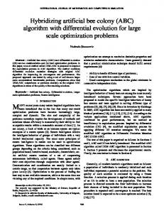
Figure 1. Convergence Graph for Function 1-5 -1-

Success Perf.

le~~~~~~~~~~~~~~~~~~~~~~~as -se~~~~~~~~~~~~~~~~~1 "'s; ..e;,

1.0126e+004

t I

off

zZ.

........

k

le L

I

4

le r,

i i i i

lo(,0L-- I

2

i

......

5-~~~~~~~~~~~-

t

4

5 Pt

6

I

8

0

x

IC'

Figure 2. Convergence Graph for Function 6-10 Table 10. Best Error Functions Values Achieved in the MAX-FES & Success Performance (30D) 13th 25t' Success Perf. F 7Ih 19", Mean Mint Std rate (Med) (Max) (Mfin) rate 1

2.023 3e+00

2.023 3e+00

2.0234 e+004

2.0234 e+004

2

1.217 Se+00

1.334 4e+00 5

1.4174 e+005

e+005

4

2.448 2e+00 5

2.843 4e+00 5

2.9639 e+005

5

-

-

-

6.964 8e+00

8.342 2e+00

1.0162 e+005

1.6748 e+005

8.299

1.035

1 .0389

1.0395

3

6

7

8 9

4

5

4

4

4

2.023

4e+00 4

1.4648

2.023 4e+00

4_

5.0662 e-001

-

1.00

2.0234e+004

_ 0.96

1.4883e+005

0

0

0.52

5.3816e+005

0

0

~~~~~~~~~~~~~~~~~~o13 -

0

0

0.80

1.3477e+005

0

5e+00

e+005

le+00

12

1.039

e+005

6e+00

9.893

464+00

9.0090

e+003

1.00

0

9.8934e4004

1

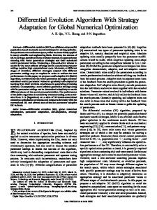
The lOD convergence maps of the SaDE algorithm on functions 1-5 functions 6-10, functions 1 1-15, functions 16-20, and functions 21-25 are plotted in Figures 1-5 respectively. The 30D convergence maps of the SaDE algorithm on functions 1-5 functions 6-10, functions 1115 are illustrated in Figures 6-8, respectively.

Figure

4

3.

5

Convergence Graph

,

,

1789

Authorized licensed use limited to: UNIVERSITY OF NOTTINGHAM. Downloaded on December 11, 2009 at 07:19 from IEEE Xplore. Restrictions apply.

71

for Function

11I-1 5

1790

.

to'

--.t1a117.

;, ,X

le, r0j

Ig r.J.

i

i.11

:

.Z-

i;

0

alst

_

I

'i

I"I.,

mm.

.l

uf

........... ...................

r0

1

4

vI

i,0&

10~~~~~~~~~~~~~~~~~~~~1

r0 0i

i~~~~~~~~E

F

W

.

r¢-

I.

05

t4

l

9

1

i

1

Zr~~~~~FE Xt

Figure 7. Convergence Graph for Function 6-10

Figure 4. Convergence Graph for Function 16-20 10; ;-W 24r

,oXhi

faal2S

-

|2~ ~ ~ ~ ~ &141

rX ke

i0t L ;

f

If

1r

IS

r¶0

10'

r.'4f -- - - ----i*

-

-

-

-*--

--r

-

--

-

-

--

-

--

-

---

-

--

-

-

0

i

05'

t1 **_w

6

2

2

{

Figure 8. CnegneGahfrFnto1-5 0\

2

5

$

4

6

$

7

6

4

%~ ~ ~ ~ ~ ~ ~ 1

i0

Oxlo'

,

Figure 5. Convergence Graph for Function 21-25 1

..

... T

ww

-

km

-_-r

t.--r.

4it

I

5.

t

*Lm

1-0

2r

W~~~~~~~~~~~-

2.$

Figure 6. Convergence Graph for Function 1-5

11

From the results, we could observe that, for lOD problems, the SaDE algorithm can find the global optimal solution for functions 1, 2, 3, 4, 6, 7, 9, 12 and 15 with success rate 1, 1, 0.64, 0.96, 1, 0.24, 1, 1 and 0.92, respectively. For some functions, e.g. function 3, although the success rate is not 1, the final obtained best solutions are very close to the success level; For 30D problems, the SaDE algorithm can find the global optimal solutions for functions 1, 2, 4, 7 and 9 with success rate 1, 0.96, 0.52, 0.8 and 1, respectively. However, from function 16 throughout to 25, the SaDE algorithm cannot find any global optimal solution for both 1 OD and 30D over the 25 runs due to the high multi-modality of those composite functions and also the local search process asscociated with the SaDE make the algorithm to prematurely converge to a local optimal solution. Therefore, in our paper, we do not list the 30D results for functions 16-25. The algorithm complexity, which is defined on http://www.ntu.edu.sg/home/EPNSugan/, is calculated on 10, 30, 50 dimensions on function 3, to show the algorithm complexity's relationship with increasing dimensions as in Table 9. We use the Matlab 6.1 to implement the algorithm and the system configurations are listed as follows:

1790

Authorized licensed use limited to: UNIVERSITY OF NOTTINGHAM. Downloaded on December 11, 2009 at 07:19 from IEEE Xplore. Restrictions apply.

1791

System Configurations Intel Pentiumg 4 CPU 3.00 GHZ 1 GB of memory Windows XP Professional Version 2002 Language: Matlab

D=10 D=30 D=50

[8] Bryant A. Julstrom, "What Have You Done for Me Lately? Adapting Operator Probabilities in a SteadyState Genetic Algorithm" Proc. of the 6th International Conference on Genetic Algorithms, pp.81-87,1995.

Table 9. Algorithm Complexity TO TI T2 (T2-TI)/TO 40.0710 31.6860 68.8004 0.8264 40.0710 38.9190 74.2050 0.8806 40.0710 47.1940 85.4300 0.9542

5 Conclusions In this paper, we proposed a Self-adaptive Differential Evolution algorithm (SaDE), which can automatically adapt its learning strategies and the asscociated parameters during the evolving procedure. The performance of the proposed SaDE algorithm are evaluated on the newly proposed testbed for CEC2005 special session on real parameter optimization.

Bibliography [1] R. Storn and K. V. Price, "Differential evolution-A simple and Efficient Heuristic for Global Optimization over Continuous Spaces," Journal of Global Optimization 11:341-359. 1997. [2] J. Ilonen, J.-K. Kamarainen and J. Lampinen, "Differential Evolution Training Algorithm for FeedForward Neural Networks," In: Neural Processing Letters Vol. 7, No. 1 93-105. 2003. [3] R. Storn, "Differential evolution design of an IIRfilter," In: Proceedings of IEEE Int. Conference on Evolutionary Computation ICEC'96. IEEE Press, New York. 268-273. 1996. [4] T. Rogalsky, R.W. Derksen, and S. Kocabiyik, in "Differential Evolution Aerodynamic Optimization," In: Proc. of 46h Annual Conf of Canadian Aeronautics and Space Institute. 29-36. 1999. [5] K. V. Price, "Differential evolution vs. the functions of the 2nd ICEO", Proc. of 1997 IEEE International Conference on Evolutionary Computation (ICEC '97), pp. 153-157, Indianapolis, IN, USA, April 1997. [6] R. Gaemperle, S. D. Mueller and P. Koumoutsakos, "A Parameter Study for Differential Evolution", A. Grmela, N. E. Mastorakis, editors, Advances in Intelligent Systems, Fuzzy Systems, Evolutionary Computation, WSEAS Press, pp. 293-298, 2002. [7] J. Gomez, D. Dasgupta and F. Gonzalez, "Using Adaptive Operators in Genetic Search", Proc. of the Genetic and Evolutionary Computation Conference (GECCO), pp.1580-1581,2003.

1791

Authorized licensed use limited to: UNIVERSITY OF NOTTINGHAM. Downloaded on December 11, 2009 at 07:19 from IEEE Xplore. Restrictions apply.