Self-adaptive Source Separation-Part II - Semantic Scholar

IEEE TRANSACTIONS ON SIGNAL PROCESSING, VOL. 46, NO. 1, JANUARY 1998

39

Self-Adaptive Source Separation—Part II: Comparison of the Direct, Feedback, and Mixed Linear Network Eric Moreau, Member, IEEE, and Odile Macchi, Fellow, IEEE

Abstract—In the first part of the present paper, we investigated stability and convergence of a new direct linear adaptive neural network intended for separating independent sources when it is controlled by the well-known Hérault–Jutten algorithm. In this second part, we study the corresponding feedback adaptive network. For two globally sub-Gaussian sources, the network achieves quasiconvergence in the mean square sense toward a separating state. A novel mixed adaptive direct/feedback network that is free of implementation constraints is investigated from the points of view of stability and convergence and compared with the direct and feedback networks. The three networks have the same (low) complexity. The mixed one achieves the best trade-off between convergence speed and steady-state separation performance, independently of the specific mixture. Index Terms— Adaptive algorithm, direct network, feedback network, mixed network, source separation.

I. INTRODUCTION

T

HIS is the second part of a two-fold paper concerned with the problem of separating a linear mixture of independent sources using self-adaptive linear networks. Source separation and its numerous applications are presented in detail in the introduction of [1, sect. I], and we rely on the reader to kindly refer to it. The model and notations are the same: is the vector of random sources, is the (invertible) mixture matrix (1) is the (noiseless) mixed observation vector, and processing matrix designed such that the vector

is the (2)

sources up to nonzero gains (grouped in restores the a diagonal matrix) and up to a permuted order (indicated by the permutation matrix ). Our work belongs to the approach of [2] and [3] using their original self-adaptation rule, even though the separation structure is changed. In Part I, we investigated a new structure for as a direct (feedforward) Manuscript received January 31, 1995; revised July 1, 1997. The associate editor coordinating the review of this paper and approving it for publication was Prof. José M. F. Moura. E. Moreau was with the Laboratoire des Signaux et Systémes (LSS), CNRS ´ Supelec University, Gif sur Yvette, France. He is now with the Groupe d’Etude des Signaux et Systémes (MS-GESSY), ISITV, La Valette du Var, France (email: [email protected]). O. Macchi is with the Laboratoire des Signaux et Systémes (LSS), CNRSSupelec-University, Gif sur Yvette, France (e-mail: [email protected]). Publisher Item Identifier S 1053-587X(98)00530-3.

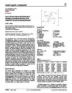
network. It is free of the realizability constraints involved in the recursive (feedback) network originally used in [2] and [3]. With a particular emphasis on the case of two sources, we have established by theory that the adaptive network algorithm is convergent in the “quasi”-quadratic mean sense toward a separating state. This paper provides the theoretical proof of convergence of the Hérault and Jutten adaptive feedback network itself. Then, we propose a third network structure, which mixes a direct part with a feedback part, while retaining the advantage of no realizability constraint. In the case of two sources, we compare the convergence speeds of the three networks at the same level of achievement in the steady state. Section II (resp., III) is devoted to the convergence analysis of the feedback (resp., mixed) structure. In both cases, an upper bound is derived for the step size under which the algorithm is stable and another bound for plain convergence. Section IV is devoted to the comparison of the three structures, both theoretically and thanks to computer simulations. Section V is our conclusion. II. THE FEEDBACK STRUCTURE REVISITED A. The Structure The feedback structure, hereafter denoted (F), has been proposed independently in 1982 by Bar-Ness et al. [4] for satellite communication and in 1984 by Hérault and Ans [2] for modeling in neurobiology. It uses linear cells with inputs and one output. The cells constitute a fully interconnected network, where the outputs of the other cells are inputs to each particular cell . The last input of cell is , with the corresponding coefficient equal to 1. Numerically, these features read (3) where is the identity matrix. The computational complexity of this structure is very low. It is only multiplications, as in the case of the direct network [1], and is less than multiplications per restored source. As explained in [1, sect. I], unless the inverse matrix is explicitly calculated (at the cost of greatly increasing the computational complexity), the implementation of the joint system (3) is not realizable. The feedback structure is depicted in Fig. 1 for sources.

1053–587X/98$10.00  1998 IEEE

40


Adaptation is usually performed in a discrete way, i.e., incremented according to

is (10)

The adaptation law for

Fig. 1. Feedback structure (F) for the case of two sources.

B. Separating States sources, there are two configurations For the case of for the mixture matrix . The first configuration occurs when (4) Then, there are two separating states. The first one is

(11)

is borrowed from [2] and [3], where for the coefficients is a positive constant step size. It is the Hérault–Jutten (HJ) algorithm. The increment is evaluated taking the previous to calculate and in (11). values Although this updating rule is not fully justified in [3], its basic advantage is that the separating states are equilibrium points of the algorithm (10), as shown below. The overall arithmetical complexity, including the adaptation, is approximately multiplications, that is, multiplications per recovered source. This is a very low computational cost. The equilibrium points of (10) are those states for which the increment is zero mean. They are the roots of the system

(5) (12) It is associated with

so that (6)

. It is associated The second one is so that , . with Remark: It is clear that with the modified quantities and , the observed vector remains unaffected. This merely amounts to relabeling the sources. This is why, without any loss of generality, it will be assumed in the following that (7) and [which is a special When case of (7)], the source dominates channel , while the dominates channel . Then, according to (6), the source separating point restores each source in the channel where it is dominant. Therefore, we call the “natural” separating state. For the same reason, the separating state is called “reversing.” The second configuration occurs when (8) is excluded because The case where would not be invertible. Thus, according to (7), , and . When (resp., ) is a lower (resp., upper) triangular matrix. Then, there is one and only one separating state, that is, the natural one . C. Equilibrium Points and Stability We relabel the coordinates with a single index , which indicates the rank of in the vector

(9)

Thanks to independence of the zero-mean variables , it is clear that (12) is satisfied when is a separating point. Separating points are equilibria of (10). Note that the converse is not true. The next issue, that is, stability of these equilibria, can be approached using the so-called ODE technique. It approximates the discrete algorithm with the help of a differential deterministic system (13) where (14) in ). The differential system (13), ( is the rank of (14) is stable in the vicinity of an equilibrium point iff its tangent linear system is stable (the matrix associated with this transformation has all its eigenvalues with a negative real part). This approach requires an infinitesimal step size. For two sources, the equilibria and their stability have been investigated in [6] and [7]. For the configuration (4) of matrix , there are four equilibria, namely, , (the two separating states) plus two nonseparating states , . In [6], it is shown that neither nor can be stable unless the fourth-order moments of sources satisfy (15) is defined by and where the positive quantity where the sources have normalized power ( ). The last condition has no loss of generality since the power of sources can be transferred into the entries of matrix . Sources for which (15) is valid are called “globally sub-Gaussian.” and are For example, this condition holds when both less than 3, which corresponds to two sources with negative

MOREAU AND MACCHI: SELF-ADAPTIVE SOURCE SEPARATION—PART II

kurtosis. Under (15), the nonseparating equilibria and are unstable [6], [7]; therefore, the adaptive algorithm will not reach these ill states. Moreover, the stability of requires that the associated coefficients satisfy or

41

For two sources, it is shown in Appendix A that the “natural” separating state is stable iff (23) (24)

(16)

It is easily seen, then, that the natural separating state does indeed satisfy the stability condition (16) for all mixture , it depends on the matrices . For the reversing state number of minus signs in . For an even number of them, is unstable. In the opposite case, both and are stable. For the configuration (8) of matrix , there are only three equilibria, namely, the separating state (which is stable) plus the two (unstable) nonseparating equilibria and .

is the determinant of matrix where . Condition (23) is the same as (15), which is found in Section II-C. Condition (24) gives the step size bound we are seeking. This bound is indeed positive thanks to (7). When the “reversing” separating state exists (i.e., no zero entry in ), the Appendix shows that it is stable iff there is an odd number of minus signs1 in and

D. Upperbounding the Step Size

is the “subComments: The stability condition Gaussian” condition already discussed in Section II-C. The upper-bounds (24) and (25) for the step size depend both on the statistics of sources and on the mixture matrix . They approach zero when becomes irregular (which is a case that is forbidden). However, they are unaffected when the statistics of sources approach the limiting situation where is null (e.g., 2 Gaussian sources).

The above analysis is not complete. First, the stability conditions that have been derived are only necessary. Second, the step size has to be small enough to ensure that the averaged discrete algorithm (17) works like the continuous one in (13). This is a drawback inherent to the ODE method. To get the upper bound over the step size , it is necessary to calculate the linear system that is tangent to (17). In the vicinity of a separating state , this system is written (18) and the matrix

using the deviation of partial derivatives with entries

Clearly, this system is stable iff all the eigenvalues of have modulus less than 1. Now, according to (14)

In this subsection, we closely follow the approach given [1, Sec. V, Pt. I] for the direct adaptive network. Consider the case of two sources, and assume that the initial state is in the attraction basin of the natural separating point . We again use the deviation . Moreover, denote

The adaptive algorithm (10), (11) reads (27)

(21)

is evaluated with an th trial of the input where sources, whereas the state of the network is . Let denote the vector similar to but with the network in the separating state . The first-order expansion of in the vicinity of the state is , where the four elements of the matrix are

is the element of the inverse matrix . Accordingly, for a separating equilibrium (where ’s are independent), one has

(28)

(20) Moreover, it follows from (3) that

distinct

E. Convergence Analysis

(26) (19)

where

(25)

if if if

Taking into account the relationships (5) and (6), it turns out that (22)

Now, it is possible, in principle, to test the stability of the tangent system (18). The procedure is to calculate the roots of the characteristic polynomial associated with and to check that all of them have a positive real part. This appears difficult, at least for greater than 2.

(29)

g g D

1 As a result of (7), the quantity 12 21 g is positive in that case; therefore, the bound (25) is indeed positive.

42


Therefore, the first-order expansion of the vector

in (26) is (30)

where we have (31), shown at the bottom of the page. It follows from (27) and (30) that the algorithm can be written (32) This is formally the same recurrence as for the direct adaptive network of [1, Eq. (80)], namely

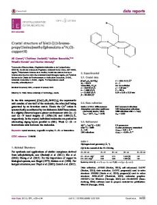
Fig. 2. Mixed structure (M) for the case of two sources.

(33) Moreover, the quantities and (which are characteristic of the feedback network) and the quantities and (which are characteristic of the direct network) are related by (34) (35) where the matrix is zero mean. Then, based on the assumption that the sequence is i.i.d.,2 it is straightforward to investigate the convergence of (32) thanks to the Appendix of Part I. 1) Convergence of the Mean of : The vector is exponentially vanishing iff the stability condition (23) holds, and the step size is upperbounded according to (24). 2) Mean Square Behavior: When increases, the covariance matrix of the deviation is exponentially convergent toward a limit that is upper bounded by a constant times the step size . This is the concept of quasiconvergence in the mean square sense (see e.g., [9, chs. 3, 6]). Moreover, for infinitesimal, is, in fact, proportional to , and using the characteristic vector , we get the result (36)

III. THE MIXED STRUCTURE A. The Structure In [8], we have presented a mixed structure where the feedback network is cascaded after the direct one. The separation task is thus distributed into two stages so that each stage has to perform only one half of the task. Unfortunately, this structure has the same realizability constraints as the feedback one. Moreover, there are some cases where the separating points are unstable. This is why another mixed structure is now considered, according to the input/output relationship (40) (resp., ) is a strictly lower (resp., upper) where triangular matrix (that is with zero diagonal entries). As a result, and are regular matrices. The superscripts and refer to the recursive and direct parts of the structure, respectively. The explicit writing of (40) is

.. .

(41)

with the help of the matrix (37) and of the vector (38) where the quantities are defined by . When and , the result (36)–(38) provides the steady-state mean square deviation (MSD) (39) 2 In

particular, this fact implies that Z1 (n)].

[A 1 (n);

V

(n

0 1) is independent of the pair

This structure has no realizability constraints because the ’s can be calculated recursively one after the other. Moreover, the computational complexity is the same as for the direct and feedback structures, that is, multiplications. When no confusion is possible, we can drop the super indices and in the notations ( ). The mixed structure, which hereafter is denoted (M), is depicted in Fig. 2 for sources. It is a partially interconnected network with cells. The first entries of cell are the outputs of the previous cells. Its th entry is with a coefficient equal to 1. The remaining entries are with . Such a structure was considered and made adaptive thanks to the so-called “boostrap” algorithm in [5]. Here, the more familiar (HJ) algorithm is preferred.

(31)


43

B. Separating States, Equilibrium States, and Their Stability

It is shown in Appendix C that stability of any of the two separating points or requires the global sub-Gaussian condition (23) ( ). Moreover, is stable iff , and

The separating states are those matrices . Therefore

for which

if

(42)

(51)

To proceed further, let us focus on the case of two sources . Then, (42) reads

(43)

where . According to (7), is nonzero. Therefore, the “natural” separating state (for which ) is characterized by the state vector

if It follows in a straightforward manner from (23) that if (resp., ) is negative, then (resp., ) is positive. Therefore, at least one of the two points and is indeed stable. Starting in its neighborhood, the algorithm will converge to it (in a certain sense), as explained in the next subsection. It is awkward to investigate stability of the nonseparating equilibria and by analysis. Fortunately, computer simulations show that both states are unstable. Therefore, the adaptive algorithm never reaches these ill states.

(44) C. Convergence Analysis which yields the restored sources (45) , there is a second separating state that recovers When the sources in reversed order

Following the same analysis as in Section II-E, we take the example of the “natural” separating state , assuming that it is stable, i.e., that is positive. Equations (26) and (27) remain true, but now, the first-order expansion of the increment in the vicinity of the state is (52) where

(46) It makes sense to keep the same (HJ) adaptation as for the recursive and direct networks

(53) and where according to (44) and (45)

(47) where and are evaluated with an th trial the input sources, whereas the state of the network is The equilibrium states are those states for which

of .

(54)

(48)

It follows from (26), (27), and (52) that the deviation obeys the recursion

Clearly, the separating states are equilibrium points. However, the converse is not true. It is shown in Appendix B that there are two other equilibria

(49) . where For the stability analysis of the average algorithm, let us denote (50)

(55) It is similar to the recursion (33), which governs the direct adaptive network (cf., [1, sect. I]), although there is no relationship such as (34) and (35) relating to and to . The sequence is assumed i.i.d. in such a way that is independent of the pair . 1) Convergence of the Mean of : Because and are zero mean, the vector obeys the deterministic recursion (56) is exponentially vanishing, According to Appendix C, provided the step size is bounded according to (51) (with ).

44


2) Mean Square Behavior: Proceeding as in the Appendix of Part I, one can show that in steady state and for infinitesimal, the covariance matrix obeys the recursion (57) where

(58) and and with the matrix given in (59), shown at the bottom of the page, the recursion (57) is equivalently written

With vectors

Therefore, when

increases, the vector

A. Comparison of (D) and (F) We refer the reader to [1, sect. I] for the results concerning the direct adaptive network (D). First, (F) and (D) have equivalent stability; for both networks, the natural separating point is stable, and the reversing one is stable iff there is an odd number of minus signs in the matrix . Clearly, it follows from the obvious relationship that the feedback and the direct networks with parameters are equivalent in the sense that their output vectors are proportional if In particular, the separating states are the same . With an adaptive structure, the increment be

(63) , will

(60)

(64) (65)

converges toward

(66)

(61)

is the increment that would control the direct In (66), network (D) equivalent to (F) if it were made adaptive in the usual way of Part I. Therefore, the adaptive feedback and direct networks will remain permanently equivalent, provided that their step sizes permanently satisfy the relationship

This result (61) corresponds to quasi convergence in the mean square sense of toward , when is sufficiently small. The steady-state MSD is the sum of the first two coordinates of . It follows by straightforward computations. In particular, when and

(67) will be very close, e.g., to the separating In steady state, state , and (67) reads

(62) When is an upper triangular matrix ( ) and , (62) is simply written . In this case, ; therefore, it follows from (39) that the feedback and mixed structure have the same MSD. This value is the same for the direct structure as a result of [1, Eqs. (107)–(109)]. In this case, the three structures have identical steady-state performance for the same step size . IV. COMPARISON OF

THE

THREE STRUCTURES

It is interesting to compare the three structures (D), (F), and (M) from the points of view of stability and convergence achievement. We shall restrict our attention to the case of two sources .

(68) Under the constraint (68), the two adaptive networks (D) and (F) have identical steady-state achievements. This is confirmed by the theoretical MSD values found in Part I: (109) for (D), and in this part, (39) for (F). This property will be checked later with computer simulations. However, even with (68), the two adaptive structures are not equivalent because in the transient phase—before steady state—the condition (67) is not fulfilled. This is why they do not have the same convergence speed. Clearly, (F) will start faster than (D) from identical initial conditions if its step-size (68) is larger than , i.e., if (69)

(59)


45

Generally, the networks are started with the initial vectors . Thus, (F) starts more quickly than (D) iff or, equivalently

In the steady state, is very close to, e.g., the separating state , and (78) reads

(70)

(79)

This situation occurs iff there is an odd number of minus signs in . Otherwise, (D) starts faster than (F). These conclusions will be checked in Section V. B. Comparison of (M) with (D) and (F) From the point of view of stability, the mixed adaptive network (M) is not equivalent to the direct and feedback ones. Indeed, its stability conditions are not only dependent on the mixture but also on the fourth moments of sources because of the expressions of and in (50). On the other hand, the stability conditions for (D) and (F) depend only on . The comparison of performance in steady state is a little awkward because the structures are not equivalent: and , except in the particular case of a triangular matrix . Moreover, there is no proportionality relationship between the output vectors, even for the separating states: No number exists such that (or ), except if is triangular. The best that can be obtained is

This number is positive as a consequence of (7). Under the constraint (79), (M) and (D) have the same steadystate performance in the sense of (71), namely, , . It is difficult to check this result with the theoretical value of the MSD whose expression for the mixed structure is rather cumbersome [cf., (62)], except in the very specific case of a triangular matrix . Then, the three structures are completely equivalent in the steady state, provided that they have identical step sizes. To compare the convergence speeds of (M) with (D) and (F), we proceed as in Section IV-B with the three step sizes adjusted to yield similar steady state performance for the zero initial state. Then, (M) starts faster than (D) and slower than (F) iff there is an odd number of minus signs in . The conclusion is reversed in the opposite case. Therefore, the initial speed of (M) always stands in between (D) and (F) for similar steady-state achievements. This conclusion is validated below with the help of computer simulations.

(71) for some nonzero numbers and . Equation (71) defines a one-to-one correspondence between the parameters and , namely (72) and with the numbers adaptive structure, the increment is

. With an (73)

V. COMPUTER SIMULATIONS 1) The Statistics of Sources: The two sources have a threelevel discrete distribution parameterized by their fourth-order moments : with probability and with probability . Their kurtosis increases from 2 to when scans the interval . The parameter in (23) decreases from 8 to 0. 2) The Mixture Matrix: Several choices that fulfill (7) have been investigated.

(74) (80)

(75) where (76) In (75), is the increment that would control the direct network (D) corresponding to (M) if it were made adaptive in the usual way [1]. Now, it follows from (72) that the Jacobian matrix for the correspondence is (77) Except in the case where is large, the matrices and are close to each other. By assimilating them, we conclude that (M) and (D) will approximately maintain the correspondence (72), provided that their step sizes permanently satisfy the equation (78)

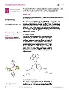
3) Stability: The first set of figures illustrates stability of the separating states. Several starting points have been chosen: the origin, the unstable separating state (when there is one), and the two unstable nonseparating equilibria and .3 The sources have identical statistics with kurtosis (that is, with probability 1/2, ). Figs. 3 and 4 exemplify the case of mixture for which both separating states are stable for the three structures. No divergence is ever observed for structure (D) (see Fig. 3). The results of structure (F) are completely similar and are omitted for the sake of brevity. Fig. 4 corresponds to structure (M), but we have plotted the state that corresponds to through (72) to help with the comparison. A divergence occurs with [whereas structure (D) converges toward with this initialization]. Figs. 5 and 6 examplify the case of 3 It is easily seen that E M (resp., E M ) corresponds to E D = E F 1 2 1 1 E2D = E2F ) in the correspondence (72).

(resp.,

46


Fig. 3. Stability of the adaptive direct network when both separating states are stable.

Fig. 4. Stability of the adaptive mixed network when both separating states are stable.

Fig. 5. Stability of the adaptive direct network when only one separating state is stable.

Fig. 6. Stability of the adaptive mixed network when only one separating state is stable.

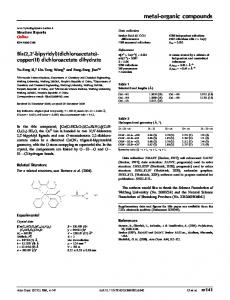
system, the positive separation index mixture for which the only stable separating state is for the direct and mixed structures, respectively. The conclusion is similar: The three structures have essentially the same stability properties. 4) Comparison of Convergence Speeds: With binary sources for the case of mixture having an odd number of minus signs, the convergence speeds of the parameters and are illustrated in Fig. 7 with similar steady-state achievements for the three algorithms. Again, the state of the mixed structure is represented by the corresponding . The analytical results are thoroughly confirmed: point (F) is superior to (M), and (M) is superior to (D). Fig. 8 with an even number of illustrates the case of mixture minus signs. Then, the conclusion is reversed. 5) Steady-State Achievement: To measure how close the overall matrix —that is, the mixture , followed by the separating network (D), (F), or (M)—is to a truly separating

(81)

have is used. The first part is zero iff all the rows of one and only one nonzero component, whereas the second is zero iff part is similar for the columns. Hence, , where is an invertible diagonal matrix, and is a permutation matrix. This corresponds to separation. Proximity to a separating state is thus characterized by vanishingly small. Figs. 9 and 10 illustrate the decrease for the three structures. The former figure with time of with an odd number of minus corresponds to the matrix signs. Again, we find the result that (F) is superior to (D)


Fig. 7. Compared convergence speed of the three structures. The case of two stable separating states.

Fig. 8. Compared convergence speed of the three structures. The case of a single stable separating state.

and that (M) stands in between. The latter figure illustrates the reversed result, using the matrix with an even number of minus signs. The mean steady-state index reaches a satisfactory level as low as 30 dB for and 35 dB for . 6) Influence of the Statistics of Sources: Finally, we have compared the separation achievements with the mixture and different values of the parameter . Fig. 11 corresponds to the case of ( and ). Compared with Fig. 10, where ( ), the convergence time is increased by 1000 iterations, and the performance incurs a loss of 10 dB in the steady state. Fig. 12 corresponds to the still smaller value ( ). Compared with the case of , the convergence time is increased by another 1500 iterations for the direct and feedback structures, but it is drastically decreased for the mixed structure. The final performance index remains unaffected ( 27 dB). In this case, the mixed structure is the most efficient one.

47

Fig. 9. Compared separation performance indices of the three structures. The case of two stable separating states.

Fig. 10. Compared separation performance indices of the three structures. The case of a single stable separating state.

VI. CONCLUSION The present contribution is the second part of a twofold paper about separation of independent sources, using self-adaptive linear networks controlled with the well-known Hérault–Jutten adaptation law. For three different structures involving similar cells and having the same very low computational complexity, we have compared stability, convergence to a separating state, steady-state separation achievement, and convergence speed both analytically and through computer simulations. The first structure is the direct network with feedforward cells. It has no realizability constraint but can have low convergence speed if there is an odd number of minus signs in the mixture matrix . The second structure is the feedback network for which the Hérault–Jutten algorithm was originally introduced. This structure has two drawbacks. First, it can have low convergence speed if there is an even number of minus signs in . Second, it involves awkward implementation constraints for the feedback. The third structure is a mixed direct/feedback

48


Fig. 11.

Influence of the statistics of sources:

= 5.

Fig. 12.

network that is free of realizability constraints. It has the advantage of a good convergence speed, independent of the signs of the entries of . Its superiority is even improved when the kurtosis of sources increases. Concerning stability, the three structures are essentially equivalent. The major feature is an upperbounding condition on fourth-order moments (kurtosis) of sources. As a result, when both sources have super-Gaussian statistics (positive kurtosis), the three adaptive structures are unstable. If both sources are subGaussian (or “globally” sub-Gaussian), there is at least one stable separating state. Depending on the entries of (as well as on the kurtosis of sources for the mixed structure), there may be a second stable separating state. Unfortunately, in the case of a single stable separating state and with certain initial conditions, divergence of the network has been observed. Yet the standard initialization putting the network parameters at the origin never yields instability. When the kurtosis of sources become large,4 the mixed structure appears to be the most efficient. For the three structures, we have proved (quasi)convergence in the mean square sense of the network toward an optimal separating state subject to suitable initialization in the attraction basin of this state. The adaptive network structure investigated in this paper has two advantages compared with other adaptive structures: it has the lowest computational complexity, and it can separate, from other sources, a source that is Gaussian or even superGaussian.

APPENDIX A

Influence of the statistics of sources:

First, consider the natural separating state of (5), (6), and (22), we get

trace

4 For two sources with the same kurtosis (hence sub-Gaussian), it means that this kurtosis is close to zero; therefore, their statistics are close to Gaussian (at fourth order).

. With the help

(84) Therefore, trace whereas

, where

, and is defined in (23),

(85) According to (82) and (83), one obtains the conditions (86) (87) If

is nonpositive, then

is positive; therefore (88)

Thus, must be positive; see (23). This means that in (86) is negative. This case has to be excluded. Hence, the . Then, the formal expression of depends condition on the value of . First Case: . Then, expression (88) holds, which means that should be positive for (87) to be valid. In this case, (86) requires that . Since , the only condition is (23). Second Case: . Then, . It has two roots:

It is well-known that the eigenvalues of the (2, 2) matrix have moduli less than 1 iff (82) (83)

= 2:75.

(89) When to

is negative, then

, and (87) is equivalent (90)

Now, it is easily seen that (91)


49

Thus, (90) is impossible. This means that must be positive: Equation (23) is required. When it is indeed satisfied, (87) reads

Replacing the factorized as

by their expressions in (93),

can be

(92) . Now, the second range is not admissible because or it comes after the instability range . In this second case, (91) and (92) are combined into the condition . In view of (85) and (89), we thus obtain the result (24) stated in the text. For the reversing separating state , the reasoning is identical, but is replaced with .

The roots of (99) are obvious. Introducing them in (96), one obtains four equilibrium points. Two of them are the separating points, whereas the two others are the points and given in (49). They are nonseparating states.

APPENDIX B

APPENDIX C

(99)

built up with the First, we compute the matrix partial derivatives of the mean algorithm increment versus the parameters and . It follows from (41) that

With notations

(100) Therefore, (47) implies that (101) It follows from (45) and (46) that (93) the system (48) of two equations with the two unknowns can be written

(102)

, (103) (94) (95)

From (94), the expression of easily derived as

as a function of

As mentioned in Appendix A, stability of the algorithm at the ( ) occurs iff separating state

is

(96)

trace

(104) (105)

With the help of (102) and (103), it is not difficult to show that (106)

Now, introducing this in (95) leads to

trace (97)

where

(107)

and where is the quantity defined in (23), whereas are defined in (50). According to (104) and (105), one obtains the conditions f

(108) (109)

(98)

These inequalities are essentially the same as inequalities (86) and (87) in Appendix A. Taking similar steps, we thus arrive easily at the result stated in Section III-B that and must be positive for the state to be stable, whereas the step size should be upperbounded according to (51).

50


REFERENCES [1] O. Macchi and E. Moreau, “Self-adaptive source separation—Part I: Convergence analysis of a direct linear network controlled by the Hérault–Jutten algorithm,” IEEE Trans. Signal Processing, vol. 45, pp. 918–926, Apr. 1997. [2] J. Hérault and B. Ans, “Réseaux de neurones a` synapses modifiables: Décodage de messages sensoriels composites par apprentissage non supervisé et permanent,” C.R. Acad. Sc. Paris, t.299, série III, no. 13, pp. 525–528, 1984. [3] C. Jutten and J. Hérault, “Blind separation of sources, Part I: An adaptative algorithm based on neuromimetic architecture,” Signal Process., vol. 24, pp. 1–10, 1991. [4] Y. Bar-Ness, J. W. Carlin, and M. L. Steinberger, “Bootstrapping adaptive cross-pol canceller for satellite communication,” in Proc. ICC Int. Conf. Commun., Philadelphia, PA, June 1982. [5] A. Din¸c and Y. Bar-Ness, “Convergence and performance comparison of the three different structures of bootstrap blind adaptive algorithm for multisignal co-channel separation,” in Proc. MILCOM, 1992, pp. 913–918. [6] E. Sorouchyari, “Blind separation of sources, Part III: Stability analysis,” Signal Process., vol. 24, pp. 21–29, 1991. [7] J. C. Fort, “Stabilité de l’algorithme de séparation de sources de Jutten et Hérault,” Traitement Signal, vol. 8, no. 1, pp. 35–42, 1991. [8] E. Moreau and O. Macchi, “Two novel architectures for the self-adaptive separation of signals,” in Proc. ICC IEEE Int. Conf. Commun., Geneva, Switzerland, May 1993, vol. 2, pp. 1154–1159. [9] O. Macchi, Adaptive Processing: The Least Mean Squares Approach With Applications in Transmission. Chichester, U.K.: Wiley, 1995.

Eric Moreau (S’93–M’96) was born in Lille, France, in 1964. He graduated from the Ecole Nationale Supérieure des Arts et Métiers (ENSAM), Paris, France, in 1989 and received the Agrégation de Physique degree from the Ecole Normale Supérieure de Cachan, Cachan, France, in 1990. He received the M.Sc. degree in 1991 and the Ph.D. degree in 1995, both in the field of signal processing from the University of Paris-Sud, Paris, France. Since 1995, he has been with the Institut des Sciences de l’Ingénieur de Toulon et du Var (ISITV), La Valette du Var, France, as an Assistant Professor and with the Groupement d’Etude des Signaux et Systèmes (MSGESSY). His main research interests are in statistical signal processing and multidimensionnal signal processing using high order statistics.

Odile Macchi (M’75–SM’84–F’89) was born in 1943 in Aurillac, France. She ´ graduated from the Ecole Normale Supérieure, Paris, France. She received the Master’s degree in both physics and mathematics in 1964 and 1965, respectively, and received the teaching degree “Agrégation” from Paris University in 1966. She received the Doctor of Science degree in 1972. Presently, she is a Director of Research of the French National Center for Scientific Research at the Laboratoire des Signaux et Systémes of the Ecole ´ Supérieure d’Electricit´ e in the field of adaptive communications, signal, and image digital processing. Dr. Macchi was awarded three French prizes in the field of electricity and was nominated Distinguished Lecturer for 1994–1995 by the IEEE Signal Processing Society. In 1994, she was elected a member of the French “Académie des Sciences.”