Self-Learning Routing for ZigBee Wireless Mesh ... - Semantic Scholar

Self-Learning Routing for ZigBee Wireless Mesh Networks Chia-Hung Tsai∗ , Meng-Shiuan Pan∗, Yi-Chen Lu∗ , and Yu-Chee Tseng∗† ∗ Department of Computer Science National Chiao-Tung University, Hsin-Chu, 300, Taiwan † Department of Information and Computer Engineering Chung-Yuan Christian University, Chung-Li, 320, Taiwan Email: {chiahung, mspan, luyc, yctseng}@cs.nctu.edu.tw

Abstract—ZigBee is defined to support low-rate wireless personal area networks (WPANs). It supports tree and mesh routing. Observing that both routing mechanisms have their pros and cons, this paper proposes a Self-Learning Routing (SLR) protocol, which inherits the low overhead of tree routing and the path efficiency of mesh routing. SLR contains an overhearing and a caching mechanism. It does not rely on sending any route discovery packets. Simulation results show that SLR outperforms ZigBee tree routing in path length. Our implementation results demonstrate that SLR can also decrease the end-to-end delay. Index Terms—caching, mesh network, routing, WPAN, ZigBee.

Addr = 64 Cskip = 1

Cm = 6 Rm = 4 Lm = 3

Addr = 92 Addr = 125 W

Addr = 30

I. I NTRODUCTION The rapid progress of wireless communication and embedded micro-sensing MEMS technologies have made wireless sensor networks (WSNs) possible. A WSN consists of many inexpensive wireless sensors deployed in a field. Each sensor node can collect and store the environmental information, and communicate with neighboring nodes to support multi-hop ad hoc routing. A lot of research activities have been dedicated to WSNs, including physical and medium access layers [1][2][3], routing and transport layers [4][5][6][7], topology control [8], time synchronization [9], and localization [10][11]. For interoperability purpose, most wireless personal area network (WPAN) platforms have adopted ZigBee [12] as their communication protocols. ZigBee adpots IEEE 802.15.4 standard [13] as its physical (PHY) and medium access control (MAC) layers and solves the interoperability issues from physical layer to network, application, and security services. Some researches have dedicated to ZigBee such as data collection strategy [14] and network formation issue [15]. ZigBee supports both mesh and tree routing. The former has an AODV-like procedure to discover the shortest routing path to each destination at the cost of higher routing overheads. The latter supports memoryless routing; routing paths can be directly inferred from network addresses and no routing tables are needed. Nevertheless, routing paths could be longer. In [16], an Enhanced Hierarchical Routing Protocol (EHRP) is proposed to improve ZigBee tree routing. Also utilizing network addresses and neighbor information, EHRP take shortcuts without incurring extra overheads.

Κcoordinator ΚRouter Κend device

Addr = 0 Cskip = 31

C U

C Addr = 63 Cskip = 7

Addr = 126

Addr = 1 Cskip = 7 V

Addr = 32 Cskip = 7

Addr = 31 Addr = 33 Cskip = 1

Addr = 40 Cskip = 1 Addr = 45

Addr = 38 Addr = 39

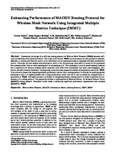
Fig. 1.

A ZigBee address assignment example.

In this paper, we propose a new Self-Learning Routing (SLR) mechanism that is more efficient than EHRP. By overhearing neighbors’ packets, nodes running SLR can gradually learn better routing paths to destinations. SLR works more like ZigBee tree routing but can take advantage of mesh routes without sending any route discovery packet. We also study the corresponding caching mechanisms to store overhearing information. Simulation and implementation results show that SLR with a proper caching mechanism can significantly outperform ZigBee and EHRP. The rest of this paper is organized as follows. Section II introduces tree-based routing defined in ZigBee. Our routing and caching strategies are presented in Section III and Section IV, respectively. Performance studies are given in Section V. Finally, Section VI concludes this paper. II. OVERVIEW OF Z IG B EE T REE ROUTING A ZigBee network consists of a coordinator and multiple routers and end devices. The network backbone is formed by the coordinator and routers, which must be IEEE 802.15.4

full function devices (FFDs). End devices can only associate with the coordinator or routers and must be reduced function devices (RFDs). ZigBee tree routing can operate relying on devices’ network addresses, which are assigned by a distributed scheme. When assigning addresses, a coordinator/router can have at most Cm children, among which at most Rm children can be routers. The depth of the network is at most Lm. To assign network addresses, a coordinator/router will be given an address block, which can be partitioned into Rm + 1 subblocks. The last block is reserved for its child end devices. The first Rm sub-blocks are to be assigned to its Rm child routers, each of size Cskip(d), where d is the depth of the node and ( 1 + Cm × (Lm − d − 1) if Rm = 1, Cskip(d) = 1+Cm−Rm−CmRmLm−d−1 otherwise. 1 − Rm (1) Address assignment begins from the coordinator by assigning address 0 to itself and depth d = 0. For a node at depth d with address Aparent , it will assign address Aparent + Cskip(d) × (i − 1) + 1 to its i-th child router and address Aparent + Cskip(d) × Rm + i to its i-th child end device. An example of the ZigBee address assignment is shown in Fig. 1. The node c is the ZigBee coordinator and the nodes which have lighter color and darker colors are represented as router nodes and end devices respectively. The Cskip of the ZigBee coordinator can be determined as 31 from Eq. (1) by setting d = 0, Cm = 6, Rm = 4, and Lm = 3. Then the 1st, 2nd, and 3rd child routers of the coordinator will be assigned to addresses 0+(1−1)×31+1 = 1, 0+(2−1)×31+1 = 32, and 0+(3−1)×31+1 = 63, respectively and they are denoted as u, v, and w in Fig. 1. There are two end devices associated with the coordinator and their address are 0+4×31+1 = 125 and 0 + 4 × 31 + 2 = 126, respectively. Based on the ZigBee address assignment scheme, the ZigBee network can easily form a tree topology. In tree routing, packets can be easily sent along the tree backbone without using any route discovery. When a node A at depth d receives a packet to node Adst , if Adst is A or one of A’s child end devices, the packet can be processed directly. Otherwise, if A < Adst < A + Cskip(d − 1), jthis packet will k be relayed −(A+1) to the child router Ar = A + 1 + Adst × Cskip(d). Cskip(d) Else, the packet will be forwarded to A’s parent. Furthermore, given a source Asrc and a destination Adst , the distance P (Asrc , Adst ) between them can be computed as follows:

Address 0x02 node hops to D P

4

R

6

P

relay table of C via to hc R

D

2

R

E

1

Address 0x04

Address 0x00

Q

C

neighbor table of R node hops to D

Cm = 2 Rm = 2 Lm = 6

Address 0x03

Address 0x01

neighbor table of C

C

5

P

4

Q

1

E

1

R

Address 0x06

D

E Address 0x40 Data(R, D, 2, E) tree link communication link send packet transmission range

relay table of R via to hc

Fig. 2.

Address 0x05

An example of SLR.

nodes that have bidirectional links with v. The relay table has entries of the format (via, dest, hc), where via is a neighboring node of v, dest is a node that can be reached via via, and hc is the hop count between via and dest. How to maintain the relay table will be addressed in Section IV. When a node v wants to send a packet to a destination d, v will compute the relay node Rnext . If d is in v’s neighbor table, it sets Rnext = d. Otherwise, it computes Rnext as follows: 1) It first examines its neighbor table. For each node x in v’s neighbor table, it computes the distance P (x, d) between x and d by Eq. (2). Then we let Rnext be the x such that P (x, d) is minimum. 2) Next, v checks its relay table and tries to find an entry (via, to, hc) such that hc + P (to, d) < P (Rnext , d). If so, it updates Rnext to via. If there are multiple candidates, the one with the smallest hc + P (to, d) is selected. Note that Step 2 implies a path v → via → · · · → to → · · · → d. Our experience shows that SLR can find a lot of shortcuts to desired destinations. Fig. 2 shows an example. To send a packet from C to D, C computes the distance from each of its two neighbors to D. The result will be Rnext = P . This gives two hops of improvement from tree routing. Now suppose that C has learned an entry of (R, D, 2) in its relay table by overhearing. Then, by applying the Step 2, Rnext will be set to R to further reduce the hop count to 3.

P (Asrc , Adst ) = D(Asrc )+D(Adst )−2×D(LCA(Asrc , Adst )), IV. C ACHING S TRATEGY (2) where D(A) is the depth of node A, and LCA(Asrc , Adst ) is In SLR, relay tables act an important role. Assuming that the least common ancestor of Asrc and Adst . the relay table is a small cache, we address the corresponding caching strategy. We start with the packet format. To facilitate III. S ELF -L EARNING ROUTING (SLR) overhearing, each data packet should carry the following SLR does not send route discovery packets. It routes packets format: Data(src, dest, hc, relay, payload), where src is the solely based on network addresses and overhearing. Each node sender, dest is the destination, hc is the hop count to dest, and v maintains two tables. The neighbor table contains those relay is the receiver of the packet. One important property of

V. P ERFORMANCE E VALUATIONS A. Simulation Results In order to justify our results, we compare SLR against the ZigBee tree routing and EHRP [16]. The ZigBee tree routing is used as a basis. Also, the optimal case will be represented by AODV protocol. The simulated network field is a 400 × 400 m2 square region and nodes are randomly deployed on this area. The tree is always rooted at the center. We set Cm = Rm = 3 and Lm = 10. The transmission range of each node is 35 m. We randomly generate sourcedestination pairs with network size setting from 500 nodes to

0.6

Saved path length ratio

0.5 0.4 0.3 0.2 EHRP vs Tree SLR with greedy caching vs Tree AODV vs Tree EHRP vs SLR with greedy caching

0.1 0 400

600

Fig. 3.

800 1000 1200 1400 1600 1800 2000 2200 Networks size Comparison of path length ratios.

0.5

Saved path length ratio

our scheme is that it is always possible to know the distance to the destination. This is the key to make overhearing feasible. When a node v receives a data packet Data(src, dest, hc, relay, payload), v can learn two things: 1) It is aware of the path length to dest is hc + 1 by going through node src. 2) It is aware of the path length to relay is 2 by going through node src. From this, v will learn two potential entries (src, dest, hc) and (src, relay, 2) to be added to its relay table. Below, we propose a greedy caching strategy to address how to update v’s relay table. Let (via, to, hc) be an entry learned by node v. The greedy strategy works as follows. 1) If there exists any entry (via′ , to, hc′ ) in its relay table with the same to and hc′ > hc, this entry will be replaced by the new one (via, to, hc). 2) Otherwise, if the relay table is not full, we directly add (via, to, hc) into the relay table. If the relay table is full, we will replace the least recently used one. If there are multiple candidates, the one with the least benefit will be replaced, where the benefit of an entry (v ′ , t, h) is defined as P (v ′ , t) − hc. For example, in Fig. 2, each neighbor of R can overhear Data(R, D, 2, E, payload) when R sends out its packet. For node C, it will learn two entries: (R, D, 2) and (R, E, 1). Since P (C, D) = 4 and P (C, E) = 6, these two entries will be inserted into C’s relay table. There are two cases that may cause SLR to fail: 1) The unstability of wireless links, which may cause the node via in some cache entry temporally unreachable. We call this a stale cache. 2) Due to cache replacement, some routing paths may be lost in the middle. To overcome these problems, we need to add one more field, mode, in each DATA packet. There are two possible values for mode: “mesh” and “ehrp”. The default value is “mesh”. When node via receives a packet with mode = “mesh”, it computes the next forwarder with hop count, says hc′ . If hc′ ≥ hc, where hc is the original value carried by the packet, via will assume that there exists a stale cache and switch to the “ehrp” mode. When entering the “ehrp” mode, the selection of Rnext will only be determined by the first rule of SLR. The mode field will be changed to “ehrp”. Then, all the rest of the forwarders will apply the same “ehrp” mode.

50% link failure rate 40% link failure rate 30% link failure rate 20% link failure rate 10% link failure rate 0% link failure rate

0.45 0.4 0.35 0.3 0.25 10

20

30

40

50

60

70

80

90

100

Relay table size Fig. 4. The impact of the relay table size on path length ratio at various link failure rates (SLR with greedy caching vs. tree routing).

2100 nodes and inject a packet from each source. Each node’s relay table is limited to 100 entries (which require 500 bytes of memory). Fig. 3 compares the ratio of the average path length of each protocol as opposed to that of the ZigBee tree routing. It shows that SLR with greedy caching can achieve over 40% of improvements over ZigBee tree routing and perform close to AODV (while incur no routing discovery overhand and incur low memory burdens). Besides, SLR with greedy caching outperforms EHRP over 20%. In addition, SLR with greedy caching can benefit more as the network becomes denser because overhearing can learn richer information. In the next simulation, we take the influence of stale cache into consideration by including link failure rate. We fix the node number to be 1000 and randomly generate sourcedestination pairs. The modification in Section IV is applied. Fig. 4 shows that a higher link failure rate indeed reduces of the benefit of SLR. However, SLR with greedy routing still outperforms ZigBee tree routing over 30% even with a 50% link failure rate. Fig. 4 also shows an interesting result that the relay table size should be kept smaller when the link fail rate

ACKNOWLEDGMENT Y.-C. Tseng’s research is co-sponsored by MoE ATU Plan, by NSC grants 96-2218-E-009-004, 97-3114-E-009-001, 972221-E-009-142-MY3, and 98-2219-E-009-005, by MOEA 98-EC-17-A-02-S2-0048, and by ITRI, Taiwan. R EFERENCES

Fig. 5.

Network monitoring user interface.

is high, and larger when the rate is low (because a larger cache could contain more stale information when links are unstable). B. Real Implementation Results We have also implemented ZigBee tree routing and SLR with greedy caching on the Jennic JN-5121 platform [17]. JN-5121 has an IEEE 802.15.4 protocol stack. Our prototype allows us to randomly deploy 20 nodes in a 20 × 20 m2 indoor environment. We set Cm = Rm = Lm = 5. In our experiment, we randomly choose 10 source-destination pairs and generate 100 packets from each source at a rate of 1 packet/sec. The experiment results show that when using ZigBee tree routing, the average end-to-end delay is about 8.4 ms with an average path length of 6 hops. When using the SLR, the average end-to-end delay is about 4.1 ms with an average path length of 2 hops. Therefore, compared to tree routing, SLR can have almost 50% improvements on end-toend delay. Fig. 5 is our network monitoring tool which also can verify our implementation results. Through this tool, we can obtain the network tree topology, neighboring tables, relay tables, and routing paths. In Fig. 5, we can see that nodes really adopts the SLR to take shorter routes (dark links are the tree links and purple links are the SLR routing links). VI. C ONCLUSIONS We have proposed a novel self-learning routing protocol which is backward compatible with ZigBee routing. It does not rely on routing discovery and only utilizes overhearing to update nodes’ neighbor tables and relay tables to find shorter routing paths. SLR is more suitable for wireless sensor networks, which have resources stringent. By simulation and implementation results, SLR can have better performance in path length and delivery time. In the future, we can further investigate more efficient cache strategies to reduce the relay table size.

[1] S. Du, A. K. Saha, and D. B. Johnson, “RMAC: A routing-enhanced duty-cycle mac protocol for wireless sensor networks,” in IEEE International Conference on Computer Communications (INFOCOM)., 2007. [2] E. Shih, S.-H. Cho, N. Ickes, R. Min, A. Sinha, A. Wang, and A. Chandrakasan, “Physical layer driven protocol and algorithm design for energy-efficient wireless sensor networks,” in The ACM Special Interest Group on Mobility of Systems, Users, Data, and Computing (SIGMOBILE), 2001. [3] W. Ye, J. Heidemann, and D. Estrin, “An energy-efficient mac protocol for wireless sensor networks,” in IEEE International Conference on Computer Communications (INFOCOM)., 2002. [4] Q. Fang, J. Gao, L. J. Guibas, V. de Silva, and L. Zhang, “Glider: Gradient landmark-based distributed routing for sensor networks,” in IEEE International Conference on Computer Communications (INFOCOM)., 2005. [5] C. Intanagonwiwat, R. Govindan, D. Estrin, J. Heidemann, and F. Silva, “Directed diffusion for wireless sensor networking,” ACM Trans. on Networking, vol. 11, pp. 2–16, 2003. [6] T. Kim, D. Kim, N. Park, S. Yoo, and T. S. Lopez, “Shortcut tree routing in zigbee networks,” in 2nd International Symposium on Wireless Pervasive Computing (ISWPC)., 2007. [7] K. K. Lee, S. H. Kim, Y. S. Choi, and H. S. Park, “A mesh routing protocol using cluster label in the zigbee network,” in IEEE International Conference on Mobile Adhoc and Sensor Systems (MASS), 2006. [8] A. Cerpa and D. Estrin, “Ascent: Adaptive self-configuring sensor networks topologies,” IEEE Transactions on Mobile Computing, vol. 3, pp. 272–285, 2004. [9] Q. Li and D. Rus, “Global clock synchronization in sensor networks,” IEEE Transactions on Computers, vol. 55, pp. 214–226, 2006. [10] A. Savvides, C.-C. Han, and M. B. Strivastava, “Dynamic fine-grained localization in ad-hoc networks of sensors,” in Proc. of ACM Int’l Conf. on Mobile Computing and Networking (MobiCom), 2001. [11] Y.-C. Tseng, S.-P. Kuo, H.-W. Lee, and C.-F. Huang, “Location tracking in a wireless sensor network by mobile agents and its data fusion strategies,” The Computer Journal, vol. 47, 2004. [12] “ZigBee specification version 2006, ZigBee document 064112,” 2006. [13] “IEEE standard for information technology - telecommunications and information exchange between systems - local and metropolitan area networks specific requirements part 15.4: wireless medium access control (MAC) and physical layer (PHY) specifications for low-rate wireless personal area networks (LR-WPANs)(revision of IEEE Std 802.15.42003),” 2006. [14] Y. C. Tseng and M. S. Pan, “Quick convergecast in zigbee beaconenabled tree-based wireless sensor networks,” Computer Communications, vol. 31, pp. 999–1011, 2008. [15] M. S. Pan and Y. C. Tseng, “The orphan problem in zigbee-based wireless sensor networks,” in ACM/IEEE Int’l Symposium on Modeling, Analysis and Simulation of Wireless and Mobile Systems (MSWiM), 2007. [16] J. Y. Ha, H. S. Park, S. Choi, and W. H. Kwon, “EHRP: Enhanced hierarchical routing protocol for zigbee mesh networks,” IEEE Communications Letters, vol. 11, pp. 1028–1030, 2007. [17] “Jennic - wireless microcontrollers,” http://www.jennic.com/.