Self-organized and driven phase synchronization in coupled maps Sarika Jalan∗ and R. E. Amritkar† Physical Research Laboratory, Navrangpura, Ahmedabad 380 009, India.
arXiv:nlin/0210006v2 [nlin.CD] 17 Apr 2003
We study the phase synchronization and cluster formation in coupled maps on different networks. We identify two different mechanisms of cluster formation; (a) Self-organized phase synchronization which leads to clusters with dominant intra-cluster couplings and (b) driven phase synchronization which leads to clusters with dominant inter-cluster couplings. In the novel driven synchronization the nodes of one cluster are driven by those of the others. We also discuss the dynamical origin of these two mechanisms for small networks with two and three nodes. 05.45.Ra,05.45.Xt,84.35.Xt,89.75.Fb
Recently, there is considerable interest in complex systems described by networks or graphs with complex topology [1]. Most networks in the real world consist of dynamical elements interacting with each other. Thus in order to understand properties of such dynamically evolving networks, we study a coupled map model of different networks. Coupled maps show rich phenomenology that arises when opposing tendencies compete; the nonlinear dynamics of the maps which in the chaotic regime tends to separate the orbits of different elements, and the couplings that tend to synchronize them. Coupled map lattices with nearest neighbor or short range interactions show interesting spatio-temporal patterns, and intermittent behavior [2]. Globally coupled maps (GCM) where each node is connected with all other nodes, show interesting synchronized behavior [3]. Ref. [4] are some of the papers which shed light on the collective behavior and synchronization of coupled maps/oscillators with local and non-local connections on different networks.
to intra-cluster couplings in the dynamics of the difference variables while the driven behaviour has its origin in the cancellation of the inter-cluster couplings in the dynamics of the difference variables. Consider a network of N nodes and Nc connections. Let each node of the network be assigned a dynamical variable xi , i = 1, 2, . . . , N . The evolution of the dynamical variables is given by X ǫ Cij g(xjt ) j Cij
xit+1 = (1 − ǫ)f (xit ) + P
where xin is the dynamical variable of the i-th node at the t-th time step, C is the adjacency matrix with elements Cij taking values 1 or 0 depending upon whether i and j are connected or not. The matrix C is symmetric with diagonal elements zero. The function f (x) defines the local nonlinear map and the function g(x) defines the nature of coupling between the nodes. In this paper, we present the results for the local dynamics given by the logistic map f (x) = µx(1 − x) and two types of coupling functions, (i) g(x) = x and (ii) g(x) = f (x). Synchronization of coupled dynamical systems may be defined in various ways [5]. Perfect synchronization corresponds to the dynamical variables for different nodes having identical values. Phase synchronization corresponds to the dynamical variables for different nodes having values with some definite relation [6]. For networks with Nc ∼ N , we find that perfect synchronization leads to clusters with very small number of nodes, while phase synchronization gives clusters with large number of nodes. Here, we concentrate on phase synchronized clusters. We define the phase synchronization as follows [7]. Let ni and nj denote the number of times the variables xit and xjt , t = 1, 2, . . . , T for the nodes i and j show local minima during the time interval T . Let nij denote the number of times these local minima match with each other. We define the phase distance between the nodes
In this paper we study the mechanisms for synchronization behaviour of coupled maps on different networks. In particular, we concentrate on networks with small number of connections, i.e. the number of connections (Nc ) are of the order of the number of nodes (N ). Our study reveals two different ways for the formation of synchronized clusters. (a) Synchronized clusters can be formed because of intra-cluster couplings. We will refer to this as self-organized synchronization. (b) Synchronized clusters can be formed because of inter-cluster couplings. Here nodes of one cluster are driven by those of the others. We will refer to this as driven synchronization. We are able to identify ideal clusters of both types, as well as clusters of the mixed type where both ways of synchronization contribute to cluster formation. We will discuss several examples to illustrate both types of clusters. Dynamically, our analysis indicates that the self-organized behaviour has its origin in the decay term arising due
∗ †
(1)
e-mail:
[email protected] e-mail:
[email protected]
1
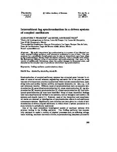
i and j as dij = 1 − 2nij /(ni + nj ). Clearly, dij = 0 when all minima of variables xi and xj match with each other and dij = 1 when none of the minima match. We say that nodes i and j are phase synchronized if dij = 0. Also, a cluster of nodes is phase synchronized if all pairs of nodes of that cluster are phase synchronized. We find examples of both self-organized and driven types of phase synchronized clusters in different networks that we have studied. For small coupling strengths, we observe turbulent behaviour, i.e. no clusters are formed, but as the coupling strength increases phase synchronized clusters are formed. The number and sizes of clusters as well as their type (self-organized, driven or mixed) depends on the coupling strength ǫ as well as the type of coupling function g(x). For networks with number of connections of the order of N , and for linear coupling g(x) = x, we observe self-organized phase synchronized clusters for small coupling strengths (ǫ ∼ 0.18) and driven phase synchronized clusters for large coupling strength with a crossover and reorganization of nodes between the two types as ǫ is increased. This behaviour appears to be approximately independent of the type of network. On the other hand, for nonlinear coupling g(x) = f (x), we observe a dominant driven phase synchronization. In this case, the sizes and number of clusters depends on the type of network for large ǫ values. As noted earlier, in this letter we concentrate only on the mechanism of cluster formation and other details will be discussed elsewhere [8]. We now present the numerical results of our model. Starting from random initial conditions and after an initial transient, we study the dynamics of Eq. (1), and determine synchronization behaviour. Fig. 1 shows several examples of clusters illustrating different behaviors. Fig. 1(a) shows two clusters with an ideal selforganized phase synchronization. We note that except one coupling, which must be present since our network is connected, all other couplings are of intra-cluster type. Fig. 1(b) shows the opposite behaviour of two clusters with an ideal driven phase synchronization. Here, all the couplings are of the inter-cluster type. Fig. 1(c) to 1(e) show mixed behaviour. Fig. 1(c) shows clusters of different types. The largest two clusters have approximately equal number of inter-cluster and intra-cluster couplings (mixed type), the next two clusters have dominant intra-cluster couplings (self-organized type) while the remaining three clusters have dominant inter-cluster couplings (driven type). Also there are several isolated nodes. Fig. 1(d) shows clusters where driven behaviour dominates. Fig. 1(e) shows clusters where self-organized behavior dominates. Fig. 1(f) shows two clusters of ideal driven type with several isolated nodes. Figs. 1(c) to 1(f) have isolated nodes which do not belong to any cluster. These nodes evolve independently, however, some of them can get attached to some clusters intermittently. To get a quantitative picture of the two ways of cluster
formation we define two quantities finter and fintra as Nintra Nc Ninter = Nc
fintra =
(2a)
finter
(2b)
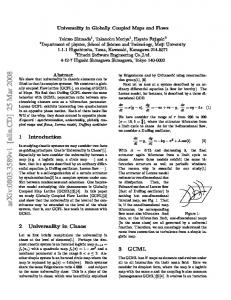
where Nintra is the number of intra-cluster couplings and Ninter is the number of inter-cluster couplings. Couplings between isolated nodes are not counted in Ninter . Figs. 2(a) and 2(b) show both fintra and finter as a function of ǫ for g(x) = x and g(x) = f (x) respectively for the scale-free networks. ¿From Fig. 2(a) (g(x) = x), we see that after an initial turbulent phase we get clusters with large values of fintra , i.e. self-organized clusters, for ǫ > 0.12. fintra becomes almost one for ǫ ∼ 0.18 ∼
and then starts decreasing. As ǫ increases further finter starts increasing and there is a crossover and reorganization of nodes to driven clusters, so that for very large ǫ, finter is close to one. The ideal driven cluster shows two driven clusters which are anti-phase synchronized with each other. On the other hand, for g(x) = f (x), Fig. 2(b) shows that finter , i.e. driven behaviour, dominates. Fig. 2(c) and 2(d) show similar graphs for network with one dimensional nearest neighbor couplings. The behaviour is similar to that of scale-free networks except that for g(x) = f (x) and for large ǫ there is almost no synchronization or cluster formation (Fig. 2(d)). It is interesting to note that the two different ways of cluster formation are observed even when the variables in the clusters are evolving chaotically. For µ = 4, we find that when three or more clusters are formed the largest Lyapunov exponent is positive. When two clusters (with or without some isolated nodes) are formed largest Lyapunov exponent can be both positive or negative depending on the parameter values and the type of coupling. If the largest Lyapunov exponent is negative, the variables show periodic behavior with even period [8]. For mu < 4, we find different periods including odd ones and also two, three or more stable clusters depending upon the parameters and initial conditions. Geometrically, the organization of the network into couplings of both self-organized and driven types is easy to understand for the networks with tree structure. A tree can always be broken into two or more disjoint clusters with only intra-cluster couplings by breaking one or more connections. Clearly, this splitting is not unique. A tree can also be divided into two clusters by putting connected nodes into different clusters. This division is unique and leads to two clusters with only inter-cluster couplings. For other types of networks splitting into clusters with ideal intra-cluster or inter-cluster couplings may not be always possible. However, clusters with dominant couplings of either intra-cluster or inter-cluster type is still possible for Nc ∼ N . For larger values of Nc , typically of the order of N 2 , a clear identification of only one 2
type of behavior becomes difficult and the clusters are mostly of the mixed type. Note that geometrically it is always possible to get one big cluster spanning almost all the nodes of the self-organized type. A comment on the choice of T used to determine the phase synchronization. Clearly, T should be large enough to include several maxima and minima. On the other hand it should be small enough to include the behavior of some isolated nodes that get attached to some clusters intermittently with a time scale of τs . We find that τs is about few thousand iterates. Hence, we chose T = 100. We have also studied networks with large N (largest N was 10,000). We can clearly identify both self-organized and driven behavior in such large networks also. To understand the dynamical origin of the selforganized and driven phase synchronization let us first consider a network of two variables, x1 and x2 , coupled to each other. Synchronization between these two variables will be decided by the difference variable xs− = x1 − x2 . From Eq. (1) the dynamics of xs− is given by
(turbulent behavior). During the match, when the match reaches a feverish pitch, i.e. the strength of the interaction increases, the fans are likely to form two driven phase synchronized groups. The response of each group depends on that of the other and is normally anti-phase synchronized with the other. Another example is the formation of opposite ethnic groups as in Bosnia. In this letter we have presented results for the case where the local dynamics is governed by logistic map and couplings g(x) = x and f (x) for the scale free networks and one-d lattice with nearest neighbor couplings. We have also studied several other maps (circle map, tent map etc.), other types of couplings and different networks (two-d lattice with nearest neighbor couplings, small world networks, Caley tree, random networks, bipartite networks). We find similar behaviour and are able to identify self-organized and driven behaviour. To conclude we have investigated the mechanism of cluster formation in coupled maps on different networks. We are able to identify two distinct ways of cluster formation, namely self-organized and driven phase synchronization. Self-organized synchronization is characterized by dominant intra-cluster couplings while driven behavior is characterized by inter-cluster couplings. The two ways of cluster formation are clearly seen for networks with small number of couplings (Nc ∼ N ) but are difficult to identify as the number of couplings increases and becomes of the order of N 2 . Dynamically, the examples of small networks show that the self-organized behaviour occurs because of the intra-cluster couplings introducing a decay term in the difference variables while the driven behaviour occurs because of the inter-cluster couplings cancelling out. One of us (REA) thanks Professor H. Kanz for useful discussions and Max-Plank Institute for the Physics of Complex Systems, Dresden for hospitality.
ǫ 1 2 2 1 xs− t+1 = (1 − ǫ)(f (xt ) − f (xt )) − (g(xt ) − g(xt ). (3) 2 Ref. [5] discusses synchronization properties of this network of two variables for g(x) = f (x). Next consider a network of three variables with both x1 and x2 coupled to x3 and no coupling between x1 and x2 . Now the dynamics of the difference xd− = x1 − x2 is given by 1 2 xd− t+1 = (1 − ǫ)(f (xt ) − f (xt )).
(4)
It can be shown that there is a critical value of ǫ above which the variables x1 and x2 will synchronize, i.e. xd− will tend to zero. The detailed dynamics of the above two simple networks and their synchronization behavior will be discussed elsewhere [8]. Comparison of Eqs. (3) and (4) clearly shows the different dynamical origins of the self-organized and driven mechanisms. The intra-cluster coupling term which is responsible for the self-organized behaviour, adds a decay term to the dynamics of xs− (Eq. (3)). On the other hand, the inter-cluster coupling terms, which are responsible for the driven behaviour, cancel out and do not add any term to the dynamics of xd− (Eq. (4)). We feel that for larger networks also similar mechanisms as in Eqs. (3) and (4) are responsible for the cluster formation of the self-organized and driven type. There are several examples of self-organized and driven behavior in naturally occurring systems. Self-organized behavior is common and is easily observed. Examples are social, ethnic and religious groups, political groups, cartel of industries and countries, herds of animals and flocks of birds, different dynamical transitions such as self-organized criticality etc. The driven behavior is probably not so common [10]. An interesting example is the behavior of fans during a match between traditional rivals. Before the match the fans may act as individuals
[1] S. H. Strogatz, Nature, 410, 268 (2001) and references therein. [2] K. Kaneko, Physica D, 34, 1 (1989), and references therein. [3] K. Kaneko, Phys. Rev. Lett. 65 1391 (1990); Physica D, 41, 137 ( 1990 ); Physica D, 124, 322 (1998). [4] H. Chate and P. Manneville, Europhys. Lett. 17, 291 (1992); N. B. Ouchi and K. Kaneko, CHAOS, 10, 359 (2000); S. C. Manrubia and A. S. Mikhailov, Phys. Rev. E, 60, 1579 (1999); P. M. Gade, H. A. Cerderia and R. Ramaswamy, Phys. Rev. E 52, 2478 (1995). [5] A. Pikovsky, M. Rosenblum and J. Kurth, Synchronization : A universal concept in nonlinear dynamics (Cambridge University Press, 2001); S. Boccaletti, J. Kurth, G. Osipov, D.L. Valladares and C. S. Zhou, Phys. Rep.,
3
[8] S. Jalan and R. E. Amritkar, unpublished. [9] A. -L. Barabasi, R. Albert, H. Jeong, Physica A, 281, 69 (2000). [10] The two sub-lattice antiferro-magnetism in statistical mechanics is also of the driven type, but it is an equilibrium phenomenon, while the driven clusters that we have are of dynamical origin.
366,1 (2002). [6] M. G. Rosenblum, A. S. Pikovsky, and J. Kurth, Phys. Rev. Lett., 76, 1804 (1996); W. Wang, Z. Liu and B. Hu, Phys. Rev. Lett. 84, 2610 (2000). S. C. Manrubia and A. S. Mikhailov, Europhys. Lett. 53, 451 (2001). [7] F. S. de San Roman, S. Boccaletti, D. Maza and H. Mancini, Phys. Rev. Lett. 81, 3639 (1998).
4
50
25
0 50
25
0 0
25
50 0
25
50 0
25
50
FIG. 1. The figure shows several examples illustrating the self-organized and driven phase synchronization. The examples are chosen to demonstrate the two different ways of obtaining synchronized clusters and the variety of clusters that are formed. All the figures show node verses node diagram for N = NC = 50. After an initial transient (about 2000 iterates) phase synchronized clusters are studied for T = 100. The logistic map parameter µ = 4. The solid circles show that the two corresponding nodes are coupled and the open circles show that the corresponding nodes are phase synchronized. In each case the node numbers are reorganized so that nodes belonging to the same cluster are numbered consecutively. (a) Figure show an ideal self-organized phase synchronization for scale free network for g(x) = x andǫ = 0.15. (b) An ideal driven phase synchronization for scale free network for g(x) = x and ǫ = 0.85. (c) Mixed behavior for 1scale free network for g(x) = f (x) and ǫ = 0.61. (d) A dominant driven behavior for scale free network for g(x) = f (x) and ǫ = 0.87. (e) A dominant self-organized behavior for 1-d lattice with nearest neighbor couplings for g(x) = x and ǫ = 0.14. (f) An ideal driven behavior with several isolated nodes for 1-d lattice with nearest neighbor couplings for g(x) = f (x) and ǫ = 0.15. The scale free networks were generated starting with N0 = 1 nodes and adding one node with m = 1 couplings at each stage of the growth of the lattice with probability of connecting to a node being proportional to the degree of the node (see Ref. [9] for details).
5
FIG. 2. The fraction of intra-cluster and inter-cluster couplings, finter (solid line) and fintra (dashed line) are shown as a function of the coupling strength ǫ. Figures (a) and (b) are for the scale free network for g(x) = x and g(x) = f (x) respectively. Figures (c) and (d) are for the 1-d network with nearest neighbor couplings for g(x) = x and g(x) = f (x) respectively. The figures are obtained by averaging over 20 realizations of a network and 50 random initial conditions for each realization.
6