Tutorials and Reviews SYNCHRONIZATION STABILITY IN COUPLED ...

Tutorials and Reviews International Journal of Bifurcation and Chaos, Vol. 10, No. 2 (2000) 273–290 c World Scientific Publishing Company

SYNCHRONIZATION STABILITY IN COUPLED OSCILLATOR ARRAYS: SOLUTION FOR ARBITRARY CONFIGURATIONS LOU PECORA and TOM CARROLL Code 6343, Naval Research Laboratory, Washington DC 20375, USA GREGG JOHNSON Code 5673, Naval Research Laboratory, Washington DC 20375, USA DOUG MAR Biomedical Engineering Department and Center for Biodynamics, Boston University, Boston MA 02215, USA KENNETH S. FINK Physics Department, Columbia U., New York, USA Received June 1, 1999; Revised September 28, 1999 The stability of the state of motion in which a collection of coupled oscillators are in identical synchrony is often a primary and crucial issue. When synchronization stability is needed for many different configurations of the oscillators the problem can become computationally intense. In addition, there is often no general guidance on how to change a configuration to enhance or diminsh stability, depending on the requirements. We have recently introduced a concept called the Master Stability Function that is designed to accomplish two goals: (1) decrease the numerical load in calculating synchronization stability and (2) provide guidance in designing coupling configurations that conform to the stability required. In doing this, we develop a very general formulation of the identical synchronization problem, show that asymptotic results can be derived for very general cases, and demonstrate that simple oscillator configurations can probe the Master Stability Function.

1. Introduction

central dynamical question is, when is such synchronous behavior stable, especially in regard to coupling strengths and connectivity in the network? Furthermore, there is increasing interest in studying the effect of varying the configuration and its effect on the synchronized state and bifurcations away from the synchronized state [Cuomo, 1993; Pérez-Villar et al., 1993; Gade et al., 1995; Wu & Chua, 1995a; Belykh & Verichev, 1996; Gade, 1996; Kocarev et al., 1996; Wu & Chua, 1996; Dmitriev et al., 1997; Hu et al., 1998; Wu, 1998b]. Many approaches have been tried in solving the synchronization problem often with emphasis on a

The increasing interest in synchronization in dynamical systems, whether chaotic or periodic, has led many people to consider the phenomenon of synchronization in large arrays or networks of coupled oscillators [Kuramoto, 1975; Fujisaka & Yamada, 1983; Pikovskii, 1984; Afraimovich et al., 1986; Kopell & Ermentrout, 1984; Volkovskii & Rul’kov, 1989; Kowalski et al., 1990; Winful & Rahman, 1990; Watanabe & Strogatz, 1993; Ashwin et al., 1994; Heagy et al., 1994a; Heagy et al., 1994b; Strogatz, 1994a, 1994b; Heagy et al., 1995; Gauthier & Bienfang, 1996; Wu, 1998a]. A

273

274 L. Pecora et al.

particular coupling scheme, but ocassionally with a view to understanding general patterns of synchronization criteria that could be applied to whole classes of oscillator networks (see e.g. [Fujisaka & Yamada, 1983; Golubitsky & Stewart, 1986; Armbruster & Dangelmayr, 1987; Pérez-Villar et al., 1993; Heagy et al., 1994b; Wu & Chua, 1994; Gade et al., 1995; Wu & Chua, 1995b; Gade, 1996; Wu & Chua, 1996; Hu et al., 1998; Wu, 1998b]). Most of the networks can be classified as a collection of identical nodes (oscillators) in which the same component is taken from each node and applied to other nodes in the network with various weights which depend on the node pairs that are coupled. The use of node components can be relaxed to a more general usage of a function of the node dynamical variables as the output of each node to be fed to the other nodes. The weights are applied to each output as a whole and are often kept constant for simplicity. We have shown that we can solve a very general form of the problem of the stability of the synchronized state in oscillators coupled as mentioned above [Pecora & Carroll, 1998; Fink et al., 1999]. We have solved this problem once and for all for any set of coupling weights and connections and any number of coupled oscillators given the particular oscillator type at each node and the functional form through which the nodes are coupled. Note: We assume nothing about the motion off the synchronization manifold since that will not affect the linear stability analysis. Although the above description of the system is rather wordy, the equations of motion and, most importantly, the variational equations used in the stability analysis have a compact form that leads quickly to a general solution of the stability problem. We call the general solution the master stability function [Pecora & Carroll, 1998]. It is this master stability function that our three-oscillator system will probe. We note that several other works by Hu et al. [1998], Gade et al. [Gade et al., 1995; Gade, 1996], have used some of the techniques we present here or similar approaches [Wu, 1998a, 1998b], especially in the application of eigenvalues of the connectivity matrix to random and star coupling configurations. Especially noteworthy is the application of graph theory to configurations of oscillators by Wu [1998a, 1998b] and Wu and Chua [1995b]. Our work independently developed the master stability function for the general case and herein we show how it can be used to predict many of the phe-

nomena and characteristics of dynamics near the synchronous state. In the following sections, we derive the variational problem leading to the master stability function (MSF) in an extremely general case. We also show how the asymptotic (large real and imaginary coupling) form of the MSF can be derived. We go on to show an experimental investigation of the MSF for R¨ ossler-like circuits which discloses the stable regions of the MSF and brings into question the appropriate stability criterion to use in real systems. We show that many other synchronization stability criteria have an associated MSF. Finally, we show that a properly constructed three-oscillator system can probe the MSF by simple variation of the couplings.

2. Stability Analysis We assume the following: (1) The coupled oscillators (nodes) are all identical, (2) the synchronization manifold is an invariant manifold, (3) the same function of the components from each oscillator is used as an output to couple to other oscillators, and (4) the nodes are coupled in an arbitrary fashion which is well approximated near the synchronous state by a linear operator. Numbers (1) and (2) guarantee the existence of a synchronization hyperplane in the phase space and number (3) makes the stability function (MSF) specific to our choice of oscillators and the output function. Number (4) is the choice of many studies of coupled systems, but note the linear coupling form is necessary only near the synchronization manifold. It can be arbitrary elsewhere. In determining the stability of the synchronous state various criteria are possible. The weakest is that the maximum Lyapunov exponent or Floquet exponent be negative. This is a universal stability standard, but it does not guarantee that there are no unstable invariant sets in the synchronous state [Ashwin et al., 1994] or areas on the attractor that are locally unstable [Pecora et al., 1995; Gauthier & Bienfang, 1996; Rulkov & Sushchik, 1997], both of which can cause attractor bubbling and bursting of the system away from synchronization when there is noise or parameter mismatch. The theory we develop below will apply to almost any criterion that depends on the variational equation of the system. Each stability criterion will lead to its own master stability function. For that reason we develop the

Synchronization Stability in Coupled Oscillator Arrays 275

theory in the context of Lyapunov exponents as a stability criterion and show in the conclusions how the other criteria can be used. Let there be N nodes (oscillators). Let xi be the m-dimensional vector of dynamical variables of the ith node. Let the dynamics for each node be x˙ i = Fi (xi , H(x)) .

(1)

H: Rm → Rm is an arbitrary output function of each node’s variables that is used in the coupling. We collect node dynamical variables in x = (x1 , x2 , . . . , xN ), and write H(x) = (H(x1 ), H(x2 ), . . . , H(xN )), i.e. H is the same for all nodes. For example, we may have “y coupling” of three-dimensional oscillator nodes by choosing H as a matrix such that H22 = 1 and all other Hij = 0. In this way the y component for each node is fed into the vector field for the ith node. At this point the actual functional dependence of F on the y components [H(x)] is left unspecified. It is this latter functional dependence that defines the connectivity and coupling strengths of the network. The N − 1 constraints x1 = x2 = · · · = N x define the synchronization manifold. To test the stability of the motion in the synchronous state we must evaluate the Lyapunov exponents of directions transverse to the synchronization manifold. We want perturbations in the transverse directions to damp out (have negative Lyapunov exponents). This requires sorting out the transverse directions from the synchronization manifold directions in the variational equation. We show how this comes about naturally in our development of a master stability function. The variational equations for the coupled system are ξ˙i = J · ξi +

N X

Dj Fi · DH · ξj .

(2)

j=1

where ξj are the (m-dimensional) perturbations of the jth node, J is the usual Jacobian of any node (the derivative with respect to the first argument of Fi , which is the same for all nodes in the synchronous state), Dj Fi is the derivative (an m × m matrix) with respect to the jth perturbation in the coupling term H(x) in Fi , and DH is the Jacobian of the coupling function evaluated at each node (which is the same for all nodes in the synchronous state).

At this stage we constrain the dependence of Fi on H(x) to be as follows. Near the synchronization manifold we want this dependence to be dominated by linear terms; thus, near synchronization each P Dj Fi should approach the form j Gij DH, where Gij is a constant m × m matrix. We also want the coupling to give equal weighting to all components of DH, that is, DH·ξj is added in Eq. (2) to the sum using a scalar weight. The latter constraint requires that Gij be a multiple of the m × m unit matrix: Gij = Gij 1m . These constraints are quite general and cover many of the coupling schemes found in the literature. With the above constraints we can write Eq. (2) in a compact form using direct products of matrices, ξ˙ = [1N ⊗ J + G ⊗ DH]ξ .

(3)

where ξ = (ξ1 , ξ2 , . . . , ξN ) is the collection of perturbations of all the coupled oscillators, G is the matrix of scalar weights, Gij and 1N is the N × N identity matrix. We will refer to G as the connection matrix. Note that manifold invariance (requirement (3) above) requires points (initial conditions) that start on the manifold to stay on the manifold. Two nearby points whose difference produces a perturbation vector ξ must stay on the manifold and, hence, the perturbation ξ must be mapped to a perturbation that is still on the manifold. Vectors on the synchronization manifold are of the (block) form (1, 1,. . . , 1). This requires the variational equation to have the same vector field components for each block corresponding to a node. That leads to the requirement that the row-sum of the linear operator in Eq. (3) be the same for each block. This P leads to j Gij = c the same number for all blocks i. The effect of this constraint is to add the same time-dependent function to the diagonal. This can be seen by rewriting the variational equation as follows ξ˙i = (J + cDH) · ξi +

N X

(Gij − cδij ) · DH · ξj . (4)

j=1

The diagonal term with the Jacobian J has an added contribution of cDH and the weights in the sum (the perenthesis factor) now have row-sum of zero. We continue to write the variational equation as Eq. (3) with the understanding that the J term may also contain a contribution of cDH and the G matrix has zero row sums.


In our previous work on the MSF [Pecora, 1998; Pecora & Carroll, 1998; Pecora et al., 1998] we assumed that G had a zero row sum. We see this is not necessary. Most coupling schemes studied in the literature use zero row sum coupling in the vector field, although we see from above that it is not necessary to have linear coupling in the vector field. The main constraints show up in the variational equation. Nevertheless, for those linearcoupling schemes we see that we only need the coupling to have equal row sums. In this case we actually have a vector field on the synchronization manifold (s = synchronized state) which has an added term, viz: x˙ i = F(xi ) +

N X

Gij H(xj ),

j=1

original equations

(5)

s˙ = F(s) + cH(s), equations on synchronization manifold That is, the motion of each node in the synchronized state is given by F + cH, not by F alone. From the above assumptions, the G matrix is constant on the synchronization manifold. This means the matrix S that diagonalizes G is a constant and can be applied directly to the variational equation, Eq. (3), at all points in the synchronization manifold. This gives us a block diagonalization of the equations of motion [Heagy et al., 1994b; Golub & Loan, 1996; Pecora et al., 1997; Pecora & Carroll, 1998]. The block diagonalization uncouples the variational equations into blocks (analogous to a mode analysis) and we are left with variational equations (6) ξ˙k = [J + γk DH]ξk , where γk is the eigenvalue of G for the kth block, k = 0, 1, 2, . . . , N − 1. For k = 0 we have the variational equation for the synchronization manifold sum being (γ0 = 0) which is required by the row P zero as the equations are now set up ( j Gij = 0). All other k’s correspond to transverse eigenvectors, so we have succeeded in separating the synchronization manifold from the other, transverse directions. We can think of these as transverse modes. We now make an important observation: For each k the form of each block [Eq. (7)] is the same with only the scalar multiplier γk differing for each. This leads us to the following formulation of the associated master stability function (MSF): We calculate the maximum Floquet or Lyapunov exponent

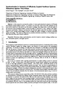
Fig. 1. Master stability function schematic. Here the stable region is the central valley with the heavy curved line separating the regions of stable (blue) and unstable (red) synchronized behavior.

λmax for the generic variational equation ζ˙k = [J + (α + iβ)DH]ξk ,

(7)

as a function of α and β (a point in the complex plane). This yields the master stability function λmax as a surface over the complex plane (see Fig. 1 as an example). Complex numbers are used since G may have complex eigenvalues. Then, given a coupling or connection matrix G we locate the point γk in the complex plane. The sign of λmax at that point will reveal the stability of that eigenmode. If all the eigenmodes are stable, then the synchronous state is stable for that coupling scheme. Interpretation of the complex coupling constant (α + iβ) may seem difficult at first, but it is easy to associate a coupling scheme each with the real and imaginary part of the MSF coupling constant. The real part is related to the symmetric part of the G connection matrix and the imaginary part is related to the antisymmetric part of G. The real part α represents a damping and the imaginary part β represents a rotation of the system between two complex conjugate eigenmodes. This is explained in more detail in [Fink et al., 1999].

3. Asymptotic Coupling Results Obviously one way to determine the MSF λmax (α + iβ) is to use traditional numerical techniques for finding Lyapunov exponents and apply them to


the generic, master variational equation (7). Here we introduce techniques that can lead to the determination of the asymptotic form of λmax for large (negative) real (α) and large imaginary (β) values. Large and negative real coupling values in Eq. (7) can sometimes be treated as follows (we set β = 0 for now). Assume the case of a constant, diagonal DH matrix, i.e. we are only coupling “like” components, xil to xjl . Then we end up with the variational equation,

simply want β large in either a positive or negative sense since the MSF must be symmetric about the real axis. For now set α = 0. As we noted above imaginary coupling amounts to a rotation. Then large β can be associated with rapid oscillations. This association will allow us to get a general asymptotic result. We assume DH is a constant, diagonal matrix with the same notation as above. This gives a variational equation,

dξ = [J + α diag{η1 , . . . , ηm }] · ξ , dt

dξ = [J + iβ diag{η1 , . . . , ηm }] · ξ , dt

(8)

The matrix diag{η1 , . . . , ηm } is DH in the form assumed above and we assume the diagonals ηi of DH are arranged in descending order (η1 > η2 > · · · ). Obviously we demand that since we are considering large, negative couplings we must have all ηi ≤ 0. If all ηi are strictly less than zero, then we automatically have the result that for large, negative real coupling α the MSF must decrease linearly ση1 . Hence, there would always be stable behavior. The case when ηj = ηj+1 = ηj+2 = · · · = ηm = 0 for some value of j is more interesting. Then we have the situation that the first j − 1 perturbation components (ξ1 , ξ2 , . . . , ξj−1 ) damp out quickly to zero values, but the stability of the last m − j + 1 components is determined by a subblock of the Jacobian J. That subblock is given by the matrix, 

Jjj  .  .  . Jmj

··· .. . ···

Note, such an equation would result if DH had a 2 × 2 antisymmetric block structure in some places along the diagonal and we diagonalized DH. We assume that for some j ηj = ηj+1 = ηj+2 = · · · = ηm = 0 whereas ηi 6= 0 for i < j. Since we can interpret iβ as causing rapid oscillation we assume a solution in the following form: ξi = φi eiβηi t

when i < j

ξi = φi

when i ≥ j

(11)

Substitution into Eq. (10) gives the following two forms of the variational equations: φ˙ i =

m X

iβ(ηl −ηi )t

Jil φl

when i < j

(12)

l=1



Jjm ..   .  Jmm

(10)

(9)

This form of the stabilty equation is obtained because the zero values of (ξ1 , ξ2 , . . . , ξj−1 ) mean the components of J with either index less than j will not contribute to the vector field of the remaining (ξj , ξj+1, . . . , ξm ) components and the zeroes of the eigenvalues will eliminate the coupling terms. Now the question of the asymptotic form of the MSF along the real axis is answered. It is a constant for small to moderate β values and its value is the largest “Lyapunov exponent” of the subblock of J [Eq. (9)]. We often refer to the subblock Lyapunov exponents as conditional Lyapunov exponents following our original work [Pecora & Carroll, 1990, 1991; Carroll & Pecora, 1991]. The case of large imaginary coupling is apparently a topic that had not been touched in the literature until [Fink et al., 1999]. First note that we

φ˙ i =

m X

lt Jil φiβη l

when i ≥ j .

(13)

l=1

Recall that β is arbitrarily large. This means the exponential terms involving β and nonzero diagonal component combinations will oscillate arbitrarily fast on the time scale of the variational system. We invoke the technique of the method of averaging for differential equations [Sanders & Verhulst, 1985] in which we can “average” in time over rapidly oscillating terms. In this case since the oscillations are so rapid the other factors are practically constant during any averaging time window and the averaging will cause any terms with nonzero exponentials to vanish. For Eq. (12) this means the only terms to survive in the sums are those for which i = l (we are assuming no degeneracy of diagonals for now). For Eq. (13) this means the only terms for which l ≥ j survive since for those, by assumption, ηl = 0. If we now allow α to be nonzero, but not large we are left with the asymptotic block form for the variational


equations:



J11 + α  0   ..   . 

 φ˙ =       

··· ··· .. .

0 0 .. .

0

···

Jj−1 j−1 + α

0

0

where φ = (φ1 , φ2 , . . . , φm ). The upper-left block is diagonal so the exponents of that block are associated with j − 1 one-dimensional variational equations. Those exponents depend on α (which is negative). The lower-right block is the same as for the large real coupling case above. In fact, as α → −∞ Eq. (14) approaches the same form as for the real case above since the exponents associated with the upper-left block will all become large and negative and only the conditional exponents of the lower-right block will matter. Thus, the imaginary asymptotic case transforms smoothly into the real asymptotic case.

4. An Application of the Master Stability Function We show an application of the MSF for the R¨ ossler system as the node system. Several configuratons of the nodes are considered, and we show the consequences of each with regard to synchronization stability can easily be seen in the MSF. dx = −(y + z) dt dy = x + ay dt

(15)

where we choose a = b = 0.2 and c = 7.0, a chaotic regime of behavior. Suppose we choose to couple our nodes using the x component. Then 1 0  H = DH =  0 0 0 0

0

··· .. . ···

Jjj .. . Jmj



0  0 0

(16)

Figure 2 shows a contour plot of the master stability function for this oscillator. We see that

Jjm .. . Jmm

       φ      

(14)

there is a region (valley) of stability defined by a roughly circular shape. The plot is symmetric in the imaginary directions about the real axis. At α = β = 0 λmax > 0 since this is just the case of isolated, chaotic R¨ ossler systems. As α increases (with β = 0) λmax crosses a threshold and becomes negative (see the cross-section of Fig. 2 in Fig. 3). Further increase in α reveals another threshold as λmax crosses over to become positive again. This implies that if the coupling is too strong the synchronous state will not be stable. This latter situation is explained by the asymptotic analysis above. When the x coupling is very strong the stability of the synchronous state will depend on the stability of the remaining y–z block (subsystem) which is easily seen to be unstable. If α is set to be in the stable range and β is increased, then λmax can also cross a threshold and become positive, implying that a large imaginary coupling can destabilize the system. The reason for this is again given by the asymptotic analysis wherein the large imaginary coupling leaves the unstable y–z subsystem controlling the synchronization stability. Diffusive coupling in a circular array adds x-coupling terms like α(xi+1 + xi−1 − 2xi ) to each node’s x ODE. The connection G matrix for this is, 

dz = b + z(x − c) dt





0 J22 + α .. .

−2 1   1 −2   1 G1 =  0  . ..  . .  . 1 0

0 ··· 1 ··· −2 · · · .. .. . . ··· 1



1 0   0  ..   . −2

(17)

and this gives eigenvalues of γk = 4 sin2 (πk/N ), each twice degenerate. The eigenmodes are discrete sine and cosine functions of the node indices i [Armbruster & Dangelmayr, 1987; Heagy et al.,


Fig. 2. Master stability function for R¨ ossler nodes with x coupling. The stable region is the central (blue) valley, the heavy curved line is the zero Lyapunov exponent line, and the unstable (red) surrounding region.

Fig. 3. Cross-section of the master stability function for x-coupled R¨ osslers. The blue line shows the stable region (the valley in Fig. 2) and the red line shows the unstable region.


1994b]. For a particular coupling strength σ we show the points σγk in Fig. 4 for an array of 10 Rösslers. The array has a stable synchronous state. As the coupling σ increases from 0, the first mode to become stable is the shortest spatialfrequency mode; the last mode to become stable is the longest spatial-frequency mode. Thus, in a stable, synchronous state, decreasing σ will cause a desynchronization with the long wavelength mode going unstable first, a long wavelength bifurcation (LWB). Increasing σ causes the shortest wavelength to become unstable, a short wavelength bifurcation (SWB) [Heagy et al., 1994b; Heagy et al., 1995] shown in the inset of Fig. 4. In this way we see that the analysis of mode stability also exposes which spatial patterns will emerge when the synchronized state loses stability in the array [Pecora, 1998]. Note, as more oscillators are added to the array, more transverse modes are created and the distance (along the real axis α) between the longest and shortest wavelength modes increases. Eventually, the system will reach a point at which we will increase σ to stabilize the long wavelength mode only to have the short wavelength mode become unstable at the same time. There will be an upper limit on the size of a stable, synchronous array of chaotic R¨ ossler oscillators [Heagy et al., 1994b; Heagy et al., 1995]. Such a size limit will always exist in arrays of chaotic oscillators with such limited stable regimes. Such a size limit will not exist if the oscillators are limit cycle, but the stable range of σ will be compressed down toward the origin as more oscillators are added to the array. In all-to-all coupling schemes (see the connection matrix G3 below) the transverse eigenvalues are all the same, γk = −σN . The all-to-all scheme can support synchronous chaos for the Rössler oscillator example for the right σ. Unlike diffusive coupling, all modes become unstable when the threshold is crossed. See Fig. 5.  −N + 1  1   1 G3 =   ..   . 1

1 −N + 1 1 .. . 1

1 1 −N + 1 .. . ···

··· ··· ··· .. . 1

 1 1    1   ..   . −N + 1

(18) Star coupling [Eq. (19)] results in two transverse eigenvalues, γk = −σ and γk = −σN . This yields two points on the master stability surface (see Fig. 6 for seven oscillators) beside the synchroniza-

tion eigenvalue. If we decrease σ, we get a desynchronizing bifurcation in which sinusoidal modes that are on the spokes of the star become unstable and grow. If we increase σ, we get an interesting desynchronization bifurcation where the nodes on the spokes remain synchronous, but the hub node begins to develop motions of opposite sign to the former. We call this a drum-head bifurcation (see the inset in Fig. 6). There is also a size limit for the star configuration. For the x-coupled Rössler example the maximum number of synchronized oscillators is 45. 

−N + 1  1    1 Gstar =   ..  .  1

1 −1 0 .. . 0

1 ··· 0 ··· −1 · · · .. .. . . ··· 0



1 0   0  ..   . −1

(19)

We now consider a more complex coupling scheme with asymmetric nearest neighbor coupling. To get the asymmetry we add an antisymmetric connection to the symmetric G1 : 

0  1   G2 =  0 . . . 1

−1 0 1 .. . 0

0 ··· −1 · · · 0 ··· .. .. . . ··· 1



1 0   0  ..   . 0

(20)

We also add all-to-all coupling, G3 . The “x” coupling term in the R¨ ossler example becomes (cs − P cu )xi+1 + (cs + cu )xi−1 − 2cs xi + ca j (xj − xi ). This is the sum of G1 , G2 and G3 . With each matrix is associated a coupling strength, cs , cu and ca , respectively. The matrices are simultaneously diagonalizable using sinusoidal modes. The eigenvalues are complex (due to the antisymmetric part), γk = −2cs [1−cos(2πk/N )]+2cu i sin(2πk/N )−ca N , and they must lie on an ellipse centered at −2cs − ca N (see Fig. 7). We can always adjust the coupling strengths so all transverse eigenvalues lie in the stable region. Increasing cs will elongate the ellipse along the real axis. Depending on where the ellipse is centered this can cause either a LWB or a SWB. Increasing cu can cause an intermediate wavelength bifurcation (IWB) for the R¨ ossler situation since the ellipse can elongate in the imaginary direction causing the intermediate wavelengths to become unstable (IWB).


Fig. 4. Master stability function showing eigenvalue placement in the complex plane for diffusive coupling where the coupling strength is set to have all the transverse modes stable. The remaining mode at α = β = 0 is the eigenvalue for the synchronization manifold. The inset shows the onset of a short wavelength bifurcation as the coupling strength is increased.

Fig. 5. Master stability function showing eigenvalue placement in the complex plane for all-to-all coupling where the coupling strength is set to have all the transverse modes which have equal eigenvalues stable. In the inset, all modes go unstable at once as the coupling strength is increased.


Fig. 6. Master stability function and eigenvalues for star coupling where the coupling strength is set to have all the transverse modes stable. In the inset, the coupling strength is increased to make the larger eigenvalue go unstable and the pattern that emerges is a growing “drum-head” mode.

Fig. 7. Master stability function showing eigenvalue placement in the complex plane for asymmetric diffusive coupling where the coupling strength is set to have all the transverse modes stable. The inset shows the onset of an intermediate wavelength bifurcation as the imaginary (antisymmetric) coupling strength is increased.


(a)

We experimentally tested the dependence of bifurcation type (LWB, IWB or SWB) as a function of couplings cs and cu using a set of eight coupled R¨ ossler-like circuits [Heagy et al., 1994a] which have individual attractors with the same topology as the R¨ ossler system in the chaotic regime. We initially set cs = 0.2, cu = 0, and ca = 0.1 so that the Rössler circuits were in the synchronous state. We controlled the coupling constants cs and cu using a digital-to-analog convertor in a computer. The circuits were started in the synchronous state and then the coupling was instantaneously reset to new values of cs and cu . At the same time, we recorded the x signals from all eight oscillators simultaneously with a 12-bit eight channel digitizer card. We arbitrarily chose the threshold of the sum of modes 1–4 exceeding 5% of the synchronous mode to determine when the oscillators were not in sync. After we switched the coupling constants cs and cu from the synchronous state to a nonsynchronous state, we fit the transient portion of each modeamplitude time series to an exponential function to find a growth rate λ for each mode. We recorded the mode with the largest λ as being the most unstable mode. Figure 8(a) shows the experimental results. In Fig. 8(b) we plot the least stable eigenmode found from the master stability function. Theory and experiment compare well. The synchronous region has a similar shape, including the sharp peak just before the SWB region. Other bifurcation regions agree reasonably well, including the small mode 3 region near the peak of the sync region.

5. The Three-Oscillator Universal Probe

(b) Fig. 8. (a) Plot of experimental results for asymmetrically coupled R¨ ossler-like circuits showing the classes of desynchronizing bifurcations that occur when the symmetric (cs ) or antisymmetric (cu ) part of the coupling is changed from a synchronous state to a state in which the theory predicts that one of the eigenmodes should be unstable. The labeling = synchronous mode, = long wavelength scheme is (mode 1), = intermediate wavelength (mode 2), = intermediate wavelength (mode 3), and = short wavelength (mode 4). (b) Similar plot of theoretical prediction of which modes are least stable.

We can calculate the MSF numerically for a great many systems so long as we have a good model for the dynamics. However, it is sometimes easier or faster to vary experimental parameters than numerical ones and in some cases the numerical model may not be accurate. In the cases where we can construct a network of the nodes we are interested in and we can control the coupling weights to each node, we now show that there is a simple configuration of three nodes that will allow us to completely probe the MSF over the entire complex plane. Consider the following setup of three coupled oscillators (we consider only additive coupling for


now for simplicity): dxi ε = F(xi ) + [H(xi+1 ) + H(xi−1 ) − 2H(xi )] dt 3 δ + √ [H(xi+1 ) − H(xi−1 )] 3 i = 1, 2, 3 cyclically

(21)

√ where we have added factors of 3 and 3 to simplify later equations. The first term is a symmetric coupling and the second term an antisymmetric coupling. The variational equation is 

J dξ  = 0 dt 0

ε  −2 3   ε δ + 3 − √ 3   ε δ +√ 3 3

6.1. Three-oscillator coupling

ε δ +√ 3 3 ε −2 3 ε δ −√ 3 3



ε δ −√  3 3  ε δ   √ + 3 3   ε  −2 3

⊗ DH · ξ .

(22)

And diagonalizing the second term connection matrix (G) gives: J 0 dψ  = 0 J dt 0 0 

0  + 0 0

6. Application of Three-Oscillator Probe to Circuit-R¨ ossler System



0 0  J 0ξ 0 J





the coupling function (H) to apply to each node, the three-oscillator system above can probe the stability of any other configuration (G) of those oscillators. In the next section we apply the universal, three-oscillator probe to a circuit version of the R¨ ossler system comparing the experimental probe of the MSF with the numerical results.



0  0ψ J 0 (ε + iδ)DH 0



0  0  ψ , (23) (ε − iδ)DH

where ψ is ξ transformed to the eigencoordinates. For the MSF, we are only interested in the lower-right 2 × 2 block. Because of the symmetry of the MSF about the real axis we only need one subblock, say for the ε + iδ block, to get the stability of the system. But we see that by varying ε and δ we can cover the entire complex plane. Hence, we can probe the entire MSF using only a three-oscillator system. For that reason we call our coupling scheme involving the three oscillators a universal probe of the master stability function [Fink et al., 1999]. It means given the node (the vector field F) and

To rigorously demonstrate the practical usefulness of the three-oscillator universal probe of the MSF, we apply the above concepts to a physical system, a system complete with inherent parameter mismatch and noise. As our chaotic oscillators, we chose to use piecewise-linear Rössler circuits as above. On the complex plane for the MSF the requirement for synchronization, the greatest Lyapunov exponent less than zero, defines a line or border. What we need now is a method to examine the stability and performance of synchronized systems on both sides of the “threshold of synchronization.” The chaotic nature of these systems makes demonstration of a synchronization threshold in a noisy physical system a particularly important step in the development of a robust theory, and yields an interesting deviation from that theory, which will be discussed later. We construct a ring of three oscillators. In the electronic implementation of the universal system of Sec. 5, voltage coupling is accomplished by a series of operational amplifiers. First, the signal from each oscillator’s x output is routed to an operational amplifier buffer; this assures that our coupling tap does not affect the operation of the running oscillators. Then, each signal is routed to three of six operational amplifier adding arrays. The first three of the six generate the (xj+1 + xj−1 − 2xj ) component, while the latter three subtract (xj+1 − xj−1). A similar scheme is used for y coupling with y j replacing xj . Finally, each signal is then multiplied by δ or ε respectively, by using an analogue multiplier IC. The time delay caused by this process is negligibly short in relation to the time scale of our oscillators.


Thus we have our fully coupled circuit equations dxj = F(xj ) + A(xj+1 + xj−1 − 2xj ) dt + B(xj+1 − xj−1 )

(24)

along with their respective variational equations dξ j = J(xj ) · ξ j + A(ξ j+1 + ξ j−1 − 2ξ j ) dt + B(ξ j+1 − ξ j−1) ,

(25)

where F is the vector field given by Eq. (21) and J is the Jacobian of Eq. (21). The matrices A and B are the symmetric and antisymmetric parts of the coupling, respectively, and are analogous to the ε and δ contributions, respectively, to Eq. (21). For x coupling the matrices A and B become 

ε  A = 0 0



0 0 0





0  0, 0

δ 0  B = 0 0 0 0

0  0 0







(26)

and for y coupling 

0  A = 0 0

0 ε 0

0  0, 0

0 0 0   B = 0 δ 0, 0 0 0

SeparationTheoretical (27)

which, except for the factors of 3, is equivalent to the G matrix of Eq. (22) when 

1  H = 0 0

0 0 0



0  0 0

which would be surpressed from observation in the coupled component since the coupling tends to slave its components to each other, regardless of what the uncoupled compenents are doing. Thus, if the uncoupled component appears to be synchronized, we can be certain that the synchronization in rest of the circuit is stable as well. We will observe the behavior of just the y component when coupling x, and observe just x when coupling y. Observations, both in numeric simulation and in physical experiment, are made in orthogonal bases perpendicular to the plane of synchronization. We have shown that the transverse directions can be given by complex numbers as in Eq. (25), but for the experiment we need real numbers so we choose two directions in real phase space that are transverse to the synchronization manifold. These are easy to find. All components are equal on the synchronization manifold which can be treated as a “vector” along the “diagonal” in phase space, namely [1, 1, 1]. Two vectors orthogonal to this diagonal, and, therefore, spanning the transverse directions, are [2, −1, −1] and [0, −1, 1]. Thus in numeric simulation for x coupling, we recorded

(28)

q

(2y 1 − y 2 − y 3 )2 + (y 3 − y 2 )2

=

(30)

In the experiment, the separation between circuits was found by capturing only two streams of data, recording (x1 − x2 ) as channel 1 (Ch1 ) and (x1 − x3 ) as channel 2 (Ch2 ). Substituting the expressions for the two channels into Eq. (30) gives, SeparationExperimental q

for x coupling and 

0

 H = 0

0

0 1 0

=



0  0 0

(29)

for y coupling.

6.2. Experimental setup Observing the stability of the circuits in the component in which we are coupling would not give a true picture of what is happening, so data must be taken from a component other than the one by which the circuits are coupled. This allows us to see any pronounced bursting or other desynchronization effects

(Ch1 + Ch2 )2 + (Ch1 − Ch2 )2

(31)

Similar results are obtained for y coupling with xj replacing y j . The experiment was controlled and automated by a LabWindows based computer program, and proceeded as follows: An 8-bit digital-to-analog converter, controlled by the computer, supplied DC voltages to the two sets of multiplier chips: one for ε, one for δ. An optimal ε and δ, determined in advance, were switched on and held for 0.1 sec (approximantely 100 cycles) insuring initial synchronization of the three oscillators. At the completion of this cycle, the voltages were simultaneously changed to new variable ε’s and δs. A


Fig. 9. Contour plot of experimental probe of the MSF (x coupling) using the synchronization distance measurement of Eq. (31). In the stable (red) region the distances were below the threshold for synchronization. In the unstable (blue) region the distances were beyond the threshold for synchronization.

few cycles later, (10−2 s), a 12-bit analog-to-digital converter began to record the separation of the oscillators, as described in the paragraph above, for approximately 400 cycles. The results were then averaged, yielding a single value for the separation of the oscillators at that particular combination of δs and ε’s.

coupling scheme (x) used in the circuits. There is no empirical link between the voltage scaling in theory and experiment, so that the scales of each may differ greatly. Within reasonable magnitudes, the shape and topology of the theory and experiment match well. Thus, we have experimentally verified the shape of the stable region of the MSF.

6.3. x coupling

6.4. y coupling

Coupling the oscillators by their x compontents, we observed the output of the y components. Figure 2 shows a map of the maximum Lyapunov exponents as predicted by computer simulation. It suggests a elliptical shape for the stable region, always with increased stability along the real line where there is no antisymmetry. Figure 9 presents the experimental version of the probe of the MSF using Eq. (31) with the same

The above process was repeated, coupling the circuits via their y components, observing the outputs of the respective x components. Figures 10 and 11 show theory and experiment respectively. As in the case of x-coupling case, the topologies and shapes generally agree with each other, but here the curvature in the synchronization threshold reveals a weakness in using the Lyapunov exponents as a measure of synchronization stability.


Fig. 10. The master stability function for y coupling in the R¨ ossler circuit.

The theoretical (Lyapunov exponent) threshold in the MSF runs almost vertically, parallel to the imaginary axis. The experimental threshold follows a parabolic shape. In the theoretical MSF such parabolic shapes occur in the contours at λmax values that are negative. This would imply that in the experiment the y-coupling arrangement needs greater stability to cause robust synchronization. We take up this subject in the conclusions.

7. Conclusions The stability of various configurations of coupled systems can now be investigated easily. The only requirement is that the variational equation (not necessarily the original evolution equations) be of the form of a “Jacobian” plus a weighted linear combination of the coupling functions to other nodes.

Here we use the word “Jacobian” to also include the extra terms added to each node’s variational equation by the coupling. We have shown that the form of the variational equation also allows one to probe the master stability function with a simple three-oscillator array whose coupling is linear and can be varied as to its symmetric and antisymmetric weights. This allows for experimental probes of the MSF giving direct contact with what would otherwise be an abstract mathematical entity. In the experimental study when we used y coupling we saw a discrepancy between the theory and experiment. In explaining that difference here we open up new possibilities for other master stability functions, each depending on the synchronization criterion one chooses. Several other criteria for synchronization thresholds have been suggested. These are (1) the maximum Lyapunov exponent or Floquet multiplier for the least stable invariant set [Ashwin et al., 1994; Rulkov & Sushchik, 1997], e.g. an unstable periodic orbit in a chaotic attractor, (2) the average of the nonconstant part of the Jacobian and coupling compared to the linear parts [Brown & Rulkov, 1997], (3) the maximum (supremum) of the real part of the eigenvalues of the (instantaneous) Jacobian (including the coupling terms) at all points or some representative set of points on the attractor [Pecora et al., 1995], e.g. when negative, this function guarantees ultimate transverse-direction contraction everywhere on the attractor, and (4) the maximum eigenvalue of the (instantaneous) symmetrized Jacobian (including the coupling terms) at all points or some representative set of points on the attractor [Gauthier & Bienfang, 1996], e.g. this guarantees monotone damping of transverse perturbations [Kapitaniak, 1996]. All criteria (1)–(4) require calculation of quantities from the same variational equation as that used here for the maximum Lyapunov exponent criterion. Hence, the same techniques that led to the block structure of the Jacobian and coupling components that we developed here will work with (1)–(4). Thus, for each criterion there is a master stability function and coupling changes will manifest themselves as motion of the eigenvalues on the complex plane just as above. Furthermore, for each criterion the analysis using the three-oscillator universal probe also holds. In this way the threeoscillator probe can be a good test for which criteria is best applicable to a particular system by


Fig. 11.

Experimental probe of the MSF (y coupling) similar to Fig. 9. (Note: Scales are not the same as Fig. 10).

comparing the experiment with the master stability function for each criterion.

Acknowledgments We thank Steve Strogatz for pointing out the generalization to nonzero row sum connections in the variational equation allowing us to generalize the master stability function approach.

References Afraimovich, V. S., Verichev, N. N. & Rabinovich, M. I. [1986] “Stochastic synchronization of oscillations in

dissipative systems,” Inv. VUZ. Rasiofiz. RPQAEC 29, 795–803. Armbruster, D. & Dangelmayr, G. [1987] “Coupled stationary bifurcations in non-flux boundary value problems,” Math. Proc. Camb. Phil. Soc. 101, 167–192. Ashwin, P., Buescu, J. & Stewart, I. [1994] “Bubbling of attractors and synchronization of chaotic oscillators,” Phys. Lett. A193, 126–139. Belykh, V. N. & Verichev, N. N. [1996] “Spatially uniform autowave processes: Global synchronization in systems with transfer and diffusion,” Radiophys. Quant. Electron. 39(5), 392–397. Brown, R. & Rulkov, N. F. [1997] “Designing coupling that guarantees synchronization between identical chaotic systems,” Phys. Rev. Lett. 78, 4189–4192.


Carroll, T. L. & Pecora, L. M. [1991] “Synchronizing chaotic circuits,” IEEE Trans. CAS. 38, 453–456. Cuomo, K. M. [1993] “Synthesizing self-synchronizing chaotic systems,” Int. J. Bifurcation and Chaos 3(5), 1327–1337. Dmitriev, A. S., Shirokov, M. & Starkov, S. O. [1997] “Chaotic synchronization in ensembles of coupled maps,” IEEE Trans. Circuits Syst. I. Fundamental Th. Appl. 44(10), 918–926. Fink, K. & Johnson, G. et al. [1999] “Three-oscillator systems as universal probes of coupled oscillator stability,” Phys. Rev. E, to appear. Fujisaka, H. & Yamada, T. [1983] “Stability theory of synchronized motion in coupled-oscillator systems,” Progress of Theoret. Phys. 69(1), 32–47. Gade, P. M. [1996] “Synchronization in coupled map lattices with random nonlocal connectivity,” Phys. Rev. E54, 64–70. Gade, P. M., Cerdeira, H. & Ramaswamy, R. [1995] “Coupled maps on trees,” Phys. Rev. E52, 2478–2485. Gauthier, D. J. & Bienfang, J. C. [1996] “Intermittent loss of synchronization in coupled chaotic oscillators: Toward a new criterion for high-quality synchronization,” Phys. Rev. Lett. 77(9), 1751–1754. Golub, G. H. & Loan, C. F. V. [1996] Matrix Computations (The Johns Hopkins University Press, Baltimore, MD). Golubitsky, M. & Stewart, I. [1986] “Hopf bifurcation with dihedral group symmetry: Coupled nonlinear oscillators,” in Multiparameter Bifurcation Theory, Contemporary Mathematics, eds. Golubitsky, M. & Guckenheimer, J. (American Mathematical Society, Providence), pp. 131–173. Heagy, J. F., Carroll, T. L. & Pecora, L. M. [1994a] “Experimental and numerical evidence for riddled basins in coupled chaotic oscillators,” Phys. Rev. Lett. 73, 3528–3531. Heagy, J. F., Carroll, T. L. & Pecora, L. M. [1994b] “Synchronous chaos in coupled oscillator systems,” Phys. Rev. E50(3), 1874–1885. Heagy, J. F., Carroll, T. L. & Pecora, L. M. [1995] “Desynchronization by periodic orbits,” Phys. Rev. E52(2), R1253–R1256. Heagy, J. F., Pecora, L. M. & Carroll, T. L. [1995] “Short wavelength bifurcations and size instabilities in coupled oscillator systems,” Phys. Rev. Lett. 74(21), 4185–4188. Hu, G., Yang, J. & Liu, W. [1998] “Instability and controllability of linearly coupled oscillators: Eigenvalue analysis,” Phys. Rev. Lett. 80(3), 496–499. Kapitaniak, T. [1996] “Monotone synchronization of chaos,” Int. J. Bifurcation and Chaos 6(1), 211–217. Kocarev, L., Parlitz, U. & Stojanovski, T. [1996] “An application of synchronized chaotic dynamic arrays,” Phys. Lett. A217, 280–284.

Kopell, N. & Ermentrout, G. B. [1984] “Frequency plateaus in a chain of weakly coupled oscillators. I,” SIAM J. Math. Anal. 15(2), 215–237. Kowalski, J. M., Albert, G. L. & Gross, G. W. [1990] “Asymptotic synchronous chaotic orbits in systems of excitable elements,” Phys. Rev. A42, 6260–6263. Kuramoto, Y. [1975] “Self-entrainment of population of coupled nonlinear oscillators,” Int. Symp. Mathematical Problems in Theoretical Physics, Lecture Notes in Physics, ed. Araki, H. (Springer, Berlin), pp. 420–422. Pecora, L., Carroll, T. & Heagy, J. [1995] “Riddled basins and other practical problems in coupled, synchronized chaotic circuits,” Chaotic Circuits for Communications, Photonics East, SPIE, Philadelphia (SPIE, Bellingham, WA). Pecora, L. M. [1998] “Synchronization conditions and desynchronizing patterns in coupled limit-cycle and chaotic systems,” Phys. Rev. E58(1), p. 347. Pecora, L. M. & Carroll, T. L. [1990] “Synchronization in chaotic systems,” Phys. Rev. Lett. 64, 821–824. Pecora, L. M. & Carroll, T. L. [1991] “Driving systems with chaotic signals,” Phys. Rev. A44, 2374–2381. Pecora, L. M. & Carroll, T. L. [1998] “Master stability functions for synchronized coupled systems,” Phys. Rev. Lett. 80(10), p. 2109. Pecora, L. M., Carroll, T. L. & Fink, K. [1998] “Stability surfaces for coupled oscillator arrays,” 1998 Int. Symp. Nonlinear Theory and its Applications, Crans-Montana, Switzerland, September 14–17, 1998 (Presses polytechniques et universitaires romandes, Lausanne, Switzerland), pp. 159–162. Pecora, L. M., Carroll, T. L., Johnson, G., Mar, D. J. & Heagy, J. F. [1997] “Fundamentals of synchronization, concepts and applications,” Chaos 7(4), p. 520. Pérez-Villar, V., Mu˜ nuzuri, A. P., Pérez-Mu˜ nuzuri, V. & Chua, L. O. [1993] “Chaotic synchronization of a onedimensional array of nonlinear active systems,” Int. J. Bifurcation and Chaos 3(4), 1067–1074. Pikovskii, A. S. [1984] “Synchronization and stochastization of array of self-excited oscillators by external noise,” Radiophys. Quant. Electron. 27(5), 390–394. Rulkov, N. F. & Sushchik, M. M. [1997] “Robustness of synchronized chaotic oscillations,” Int. J. Bifurcation and Chaos 7, 625–643. Sanders, J. A. & Verhulst, F. [1985] Averaging Methods in Nonlinear Dynamical Systems (Springer-Verlag, NY). Strogatz, S. [1994a] Nonlinear Dynamics and Chaos (Addison-Wesley, Reading MA). Strogatz, S. H. [1994b] “Norbert Wiener’s brain waves,” in Frontiers in Mathematical Biology, ed. Levin, S. (Springer, NY), pp. 122–138. Volkovskii, A. R. & Rul’kov, N. F. [1989] “Experimental study of bifurcations at the threshold for stochastic locking,” Sov. Techn. Phys. Lett. 15, 249–251.


Watanabe, S. & Strogatz, S. H. [1993] “Integrability of a globally coupled oscillator array,” Phys. Rev. Lett. 70(16), 2391–2394. Winful, H. G. & Rahman, L. [1990] “Synchronized chaos and spatiotemporal chaos in arrays of coupled lasers,” Phys. Rev. Lett. 65(13), 1575–1578. Wu, C. W. [1998a] “Global synchronization in coupled map lattices,” 1998 IEEE Int. Symp. Circuits and Systems, Monterey, CA (IEEE Press), pp. 302–305. Wu, C. W. [1998b] “Synchronization in an array of chaotic circuits coupled via hypergraphs: Static and dynamic coupling,” 1998 IEEE Int. Symp. Circuits and Systems, Monterey, CA (IEEE Press). Wu, C. W. & Chua, L. O. [1994] “A unified framework for

synchronization and control of dynamical systems,” Int. J. Bifurcation and Chaos 4(4), 979–998. Wu, C. W. & Chua, L. O. [1995a] “Application of graph theory to the synchronization in an array of coupled nonlinear oscillators,” IEEE Trans. Circuits Syst. I 42, 494–497. Wu, C. W. & Chua, L. O. [1995b] “Synchronization in an array of linearly coupled dynamical systems,” IEEE Trans. Circuits Syst. 42(8), 430–447. Wu, C. W. & Chua, L. O. [1996] “On a conjecture regarding the synchronization in an array of linearly coupled dynamical systems,” IEEE Trans. Circuits Syst. I 43(2), 161–165.