IEEE TRANSACTIONS ON SYSTEMS, MAN, AND CYBERNETICS—PART A: SYSTEMS AND HUMANS, VOL. 35, NO. 3, MAY 2005
349
Self-Organized Routing for Wireless Microsensor Networks Alex Rogers, Esther David, and Nicholas R. Jennings
Abstract—In this paper, we develop an energy-aware self-organized routing algorithm for the networking of simple battery-powered wireless microsensors (as found, for example, in security or environmental monitoring applications). In these networks, the battery life of individual sensors is typically limited by the power required to transmit their data to a receiver or sink. Thus, effective network-routing algorithms allow us to reduce this power and extend both the lifetime and the coverage of the sensor network as a whole. However, implementing such routing algorithms with a centralized controller is undesirable due to the physical distribution of the sensors, their limited localization ability, and the dynamic nature of such networks (given that sensors may fail, move, or be added at any time and the communication links between sensors are subject to noise and interference). Against this background, we present a distributed mechanism that enables individual sensors to follow locally selfish strategies, which, in turn, result in the self-organization of a routing network with desirable global properties. We show that our mechanism performs close to the optimal solution (as computed by a centralized optimizer), it deals adaptively with changing sensor numbers and topology, and it extends the useful life of the network by a factor of three over the traditional approach. Index Terms—Adaptive self-organized routing, distributed systems, mechanism design, sensor network.
I. INTRODUCTION
W
IRELESS microsensor networks provide an efficient solution to the problem of performing autonomous environmental monitoring. Large numbers of small, low-cost battery-powered sensors can be scattered randomly over a large area, where they will automatically sense and record local environmental conditions. The sensors then use low-power wireless transceivers to transmit their recorded data to a receiver or sink, where it is logged, acted upon or transmitted onwards. When making such networks operational, a key question is how to effectively manage resources such as battery life and communication bandwidth, given the dynamic nature of the system and the limited knowledge of the network topology. In such cases, the use of a central control regime becomes undesirable and thus there is much interest in investigating the use of distributed control methodologies in these networks [9],
Manuscript received May 29, 2004; revised October 8, 2004 and November 17, 2004. This research was undertaken as part of the ARGUS II DARP (Defense and Aerospace Research Partnership). This is a collaborative project involving BAE SYSTEMS, QinetiQ, Rolls-Royce, Oxford University, and Southampton University, and was supported by the industrial partners together with the EPSRC, MoD, and DTI. This paper was recommended by the Guest Editors. The authors are with the School of Electronics and Computer Science, University of Southampton, Southampton SO17 1BJ, U.K. (e-mail:
[email protected];
[email protected];
[email protected]). Digital Object Identifier 10.1109/TSMCA.2005.846382
[1]. This interest is further strengthened by the observation that beyond their immediate application, such sensor networks also serve as a model for future large-scale open computer systems in which resources, such as data storage and computational power, will be physically distributed, continually subject to changes in availability and capability, and will likely be owned by stakeholders with differing objectives [18]. Similarly, peer-to-peer systems in which services are traded amongst individual entities with no central control, share many of the same challenges [16]. To this end, in this paper, we consider the specific case of developing a distributed energy-aware routing mechanism for wireless microsensor networks. In such networks, the useful life of the entire system is determined by the battery life of each individual sensor. Since the greatest drain on these batteries is the requirement to regularly transmit recorded data to the receiver or sink, there is the potential to apply some form of network routing algorithm to reduce the power consumption of these transmissions. Typically, these routing algorithms rely on the observation that as the separation of the radio transceivers increases, the transmission power required increases geometrically. Thus, a number of short range or multihop transmissions is often more energy efficient than a single long range transmission. This, in turn, means that an efficient network can be created by having sensors act as a relay for other sensors. However, configuring this communication network is a difficult task. The sensors typically have limited localization ability and thus the topology of the network itself is unknown. This topology is also intrinsically dynamic as sensors fail, move, or are added to the network at any time. In addition, the low power radio transmissions used by such sensors are subject to interference and their propagation properties vary significantly over time. Thus there is no central point which can configure the network and sensors must use their own local information to determine who they should communicate with. The methodology that we adopt in this paper is that of mechanism design; we find a mechanism which aligns the goals of selfish individual sensors with the global goals of the entire network [4]. Such an approach develops from game theory, whereby the sensors within the network are assumed to be rational selfish agents making local decisions which increase their own utility. In traditional mechanism design settings, the individuals within the network are assumed to represent different stakeholders and “payments” are transferred between them, in exchange for services (i.e., relaying data). Here, we use the same methodology to provide a simple local decision rule that the sensors can adopt. This decision rule allows individual sensors to make local decisions based on their own local
1083-4427/$20.00 © 2005 IEEE
350
IEEE TRANSACTIONS ON SYSTEMS, MAN, AND CYBERNETICS—PART A: SYSTEMS AND HUMANS, VOL. 35, NO. 3, MAY 2005
Fig. 1. Battery-powered wireless microsensor deployed in the Briksdalsbreen glacier, Norway (actual length is 12 cm).
goals and information. The mechanism aligns the goals of the individual sensors with the overall goals of the system, thus ensuring that the network which self-organizes out of these local interactions displays desirable global properties. Specifically, the mechanism that we present provides an incentive for sensors to relay data for other sensors, but only in cases where this relaying of data will benefit the entire network. It explicitly deals with the problems of limited battery life, to ensure that the life and coverage of the sensor network as a whole are maximized and it is adaptable to external changes in both the position and the number of sensors. We compare our mechanism to two other cases: 1) the default case where sensors transmit directly to the center and 2) the optimum solution found by recasting the problem as a centralized optimization problem. In simulation, our mechanism is shown to perform close to the optimum and in comparison to the default case, extends the useful life of the sensor network by a factor of three. We demonstrate through simulation that the mechanism is robust and does not degrade significantly when we change the distribution of sensors within the network or extend the simple model of radio propagation that we use in the analysis to include probabilistic changes in the communication range of the sensors. The remainder of this paper is organized as follows. Section II describes the sensor network which we are dealing with. Section III presents the main related work in this area. Section IV presents the two parts of our mechanism: the communication protocol and the payment scheme. In Section V, we present the results of simulation experiments, and we conclude and discuss future work in Section VI. II. MICROSENSOR NETWORK Our work in microsensor networks is motivated by an e-science and pervasive computing project in which sensors have been deployed within the Briksdalsbreen glacier in Norway, to record temperature, pressure, and orientation changes over extended periods of time (see Fig. 1), [13]. However, rather than restricting our analysis to just this specific example, we consider a generic model of a sensor network. We assume that the network consists of identical sensors randomly distributed over the area to be monitored. Within this network is a single receiver or sink, that is responsible for regularly collecting data from each sensor and forwarding it on for further analysis or action. As power consumption within battery powered sensors is critical, during the design of the sensors the consumption of the electronic components required to sense and record data is typ-
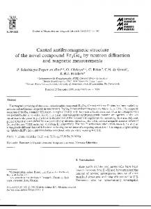
ically reduced to the minimum possible. This leaves the power used to transmit data to the sink as the deciding factor in the lifetime of the sensor. In order to model the performance of the network and to perform any analysis, we need to model the propagation of the radio transmissions between sensors and, specifically, we need to model the effect that transmission power has on communication range. Determining the degree of accuracy required for this model has been the subject of some previous research and we discuss this work further in Section III. In this paper, we start with a simple deterministic model of radio propagation, as this allows us to perform the initial analysis. We then extend this model to include probabilistic variations in the range of these radio transmissions and investigate the effect of this more realistic model. In order to simplify our model of the battery life of each sensor, we assume that the volume of the recorded data, that must be transmitted to the sink, is sufficiently large that we can ignore the power required to initially establish and negotiate the communication links. In more detail, our starting point is a simple deterministic radio propagation model in which the power to reliably transmit over a distance is proportional to the square of this distance power . To simplify future explanations, we choose the power and distance scales to remove all units and thus the lifetime of sensor , which is located at a radial distance of from the sink, is given by (1) Each sensor within the network is relatively simple and has no way of locating its own position. However, we assume that the sensors do have the ability to control the power of their radio transmissions and can thus find the minimum power necessary to transmit reliably to the receiver or sink. This ability represents the minimum necessary in order to make any attempt to maximize individual battery life and commercial radio chips are currently available with on board control of transmission power [2]. We also assume that the sensors have the ability of measuring their own power consumption and thus estimating their future battery life. We consider that the default behavior of the sensor network is that each sensor transmits its data directly to the sink at its previously found minimum power. The effect of such a policy is shown in Fig. 2, where we have assumed that sensors are randomly distributed over a circular area around the central receiver or sink. As with the radio propagation model, we revisit this assumption in Section V. In the plot, we show both the number of active sensors and the mean radius of these active sensors are plotted against time. As can be seen, no sensor has a lifetime of less than one time unit (due to the maximum radial distance of one unit); however, beyond this point, the number of active sensors rapidly decreases as sensors deplete their batteries. As those sensors that are furthest from the center deplete their batteries fastest, the mean radius of the network rapidly reduces. This has the effect of reducing the effective coverage of the sensor network to a small area immediately surrounding the sink. Against this background, our goal is to maximize not just the length of time that sensors remain active, but also the active area
ROGERS et al.: SELF-ORGANIZED ROUTING FOR WIRELESS MICROSENSOR NETWORKS
Fig. 2. Performance of the default sensor network where each sensor transmits directly to the center.
over which the sensor network is recording data (as motivated in Section I). III. RELATED WORK Routing algorithms have traditionally been based on the existence of a “routing table,” which is held at each node and is periodically updated [5]. While such methods have been successfully applied to wired networks, the additional features of the ad hoc wireless networks, on which sensor networks are based, limits their applicability. The large size of the networks, the number of potential communication routes and the time varying nature of both the network itself and its communication links, generally make such methods undesirable. Alternatives to routing tables are typically based on two techniques. The first, “on-demand” routing, maintains no route information at all, and routes are established when needed, by sending requests to forward a message [10]. Such approaches have been shown to work well on small-sized networks, where many of the messages are going to a common destination (as is the case in our example sensor network). The second techniques, geographic routing, uses the nodes physical location as an address and messages are forwarded “toward” their location using some local heuristic [7], [17]. The additional geographic information provides more efficient route discovery; however, it also introduces problems when the heuristic fails (e.g., dead-ends, where greedy routing fails to find a node closer to the destination). While traditional geographic routing demands some form of location information, work has been done to reduce this requirement. This is normally done by introducing some proxy for
351
location, such as “hop-count,” or by assigning “virtual” coordinates, which reflect the underlying connectivity of the network [3], [14]. In addition, both of these techniques have been extended to deal with energy-efficiency; typically by adding some additional transmission cost to the route information [12], [19]. The approach adopted in this paper represents a combination of these techniques. While our sensor nodes do not have full location information, we do have a proxy for this information in the form of the minimum power required to reliably communicate with the sink. As with “on-demand” routing, we allow sensors to request other sensors to forward data. However, our sensors make local decisions as to which sensors to relay data through, and use this information for subsequent transmissions. In addition, rather than simply seeking energy efficient routes through the network, our sensors explicitly take account of the limited battery life of the neighboring sensors when making these decisions. Finally, rather than relying on collaboration between sensor nodes to implement the routing algorithm, we adopt the methodology of mechanism design to provide incentives [4]. These techniques have previously been applied to routing in fixed, wired networks where the individual nodes in the network are owned by different stakeholders and generally, a payment scheme is provided that incentivizes these nodes to pass messages through the network [15], [16]. In our case, the sensors are typically all owned by the same stakeholder and this payment is unnecessary. However, the payment scheme provides a simple local decision rule which allows sensors to make local decisions, while ensuring that the actions of the individual sensors contribute to the overall goals of the systems, and it is for this reason that we adopt it here. In this respect, our approach is similar to an alternative based on statistical physics. In this case, an “energy” function or Hamiltonian is supplied to each node in the sensor network and the sensors make simple local decisions in order to minimize their own “energy” [11]. In our mechanism design approach, sensors are supplied with a payment scheme and make local decisions in order to maximize their own payments. In both cases, the decision making of the individual sensors is simplified, while the energy function and payment scheme are carefully derived to ensure that the overall system displays desirable properties. In order to actually apply this methodology to the wireless ad hoc routing found in sensor networks, a radio propagation model is required. Specifically, this model should inform us of how the communication range of the sensors is affected by their transmission power. Determining the appropriate level of accuracy of this model has been the subject of some research [8]. Specifically, Heidemann et al. compared a simple propagation model with real experimental results and found surprisingly good agreement when the sensors were deployed outside in an open environment [8]. Other results indicate that in real sensor networks the propagation properties are seen to vary stochastically over time and communication links are found to be asymmetric [20]. In addition, the transmissions of the low-power transceivers are often nonisotropic, whereby they do no radiate evenly in all directions. The results typically show long “tails,” whereby, with low probability, transmissions may be received over a much greater range than expected [6]. In this paper, we
352
Fig. 3.
IEEE TRANSACTIONS ON SYSTEMS, MAN, AND CYBERNETICS—PART A: SYSTEMS AND HUMANS, VOL. 35, NO. 3, MAY 2005
Diagram showing sensor S and potential mediator S .
adopt the methodology suggested by Heidemann et al. and perform our initial analysis on a simple propagation model. We then extend the model and confirm that our mechanism is insensitive to detail, i.e., the performance of the mechanism is robust to small changes in the underlying assumptions.
IV. MECHANISM DESIGN Our mechanism is intended to achieve two goals. First, it must provide a means for the individual sensors to make simple local decisions (i.e., who to relay data through). Second, it must ensure that these local decisions result in good global performance and increase the coverage and useful life of the sensor network. There are thus, two aspects to the mechanism. The communication protocol allows sensors to find and select a sensor that is willing to act as a mediator and relay data. The payment scheme that acts to steer the sensors to make local decisions that ensure good global performance. We discuss each separately and then go on to present simulation results indicating the performance of our mechanism. A. Communication Protocol As discussed in Section II, each sensor has the ability to find the minimum power required to reliably transmit data to the receiver or sink. Each sensor has the potential to further reduce this transmission power (and hence increase its battery life) by finding a mediator, located somewhere between itself and the sink, that is willing to relay its data. Consider the example case shown in Fig. 3 where a single sensor is seeking a mediator. We allow sensor , located a distance from the sink, to call for nearby sensors to act as a mediator. This request is transmitted at the default power level, , that sensor has previously determined is sufficient to reliably communicate with the sink and the message informs neighboring sensors of this power. Under our simple propagation model, this message will be heard by all sensors within a distance of of , and in this example, we assume that the request is heard by a sensor , which is located a distance from the sink. If willing to act as a mediator (we will discuss why it should be willing to do so in the following section), sensor responds at its own default transmission power level providing three pieces of information: its identity, its default transmission power level , and its estimated lifetime (calculated locally from observing its own battery).
Fig. 4. Diagram showing the area in which sensor S seeks a mediator under the communication protocol.
Sensors and are not able to directly measure the distance between themselves. However, as sensor has heard the response of sensor , under our deterministic radio propagawill be able communicate with sensor tion model, sensor at a power level of . Thus, if , sensor can save its battery life by transmitting at power , rather than , and relaying data through sensor . In this way, sensors are able to find neighboring sensors through whom to relay data, without explicitly needing to know their own location, or the location of other sensors. will select willing mediThus, the area in which sensor ators is illustrated as the shaded area in Fig. 4. Also shown in this figure are the positions of three potential mediators—points (1)–(3). A mediator at point (1) will be able to communicate with sensor , as both are within the range of each others’ transmissions. However, as the radial distance to the center of point (1) is greater than that of sensor , sensor will use less power by communicating directly to the center and will thus not select a mediator in this position. A mediator at point (2) is unable to communicate with sensor as although it is within range of the signal from sensor , its response is not transmitted with sufficient power to be heard by sensor . Thus, a mediator in this position, will also not be selected. However, a mediator at point (3) is able to communicate with sensor and its radial distance of the center is also smaller than that of sensor . Thus, sensor will save battery power by transmitting its data to a mediator at point (3) and will thus select a mediator in this position (or indeed, anywhere within the shaded area). Having found suitable mediators, the sensor must choose between them. In order to fully calculate the implications of using any particular sensor as a mediator, conventional routing algorithms collaboratively propagate information about new connections up and down the chain of mediators already established. Instead, we enable the sensor to make shortterm selfish decisions. The naive approach is just to select the mediator with the minimum default power level, as this minimizes the power that the sensor must use in its transmission. However, this mediator may already be acting as a mediator for several other sensors and will thus become inactive much earlier than its neighbor with a marginally greater default power level. Thus, we must also use the expected lifetime of the potential mediators when making this decision and select the mediator which appears to provide the greater increase in the lifetime of sensor .
ROGERS et al.: SELF-ORGANIZED ROUTING FOR WIRELESS MICROSENSOR NETWORKS
353
the decision making. However, the negative impact of these locally greedy decisions is lessened somewhat by allowing the sensors to find and renegotiate with mediators frequently. This ensures that information regarding the changing network structure is captured indirectly through the individual sensor’s battery consumption and reflected in their estimated lifetimes. In a dynamic environment where sensors are failing or being added to the network continually, this frequent renegotiation also allows the sensors to exploit changes in the availability of local mediators. In this context, the optimal rate of renegotiation depends on how dynamic the environment is and also on the additional factor of the overhead in time and power consumption that the negotiation represents. Thus, it is a parameter which must be tuned to the particular example scenario. B. Payment Scheme Fig. 5. Diagram illustrating the calculated increase in total lifetime of sensor S when selecting a mediator.
For example, consider the case that sensor is currently transmitting at power level and has a current estimated lifetime of . Should sensor (with expected lifetime and default power level ) act as a mediator, the increased lifetime of sensor is given by the ratio of the transmission power (2) This case is shown as case (a) in Fig. 5 and is only valid when the mediator does not become inactive within this time (i.e., ). In the more complex case, shown as case (b) in Fig. 5, the time is given by considering the fact that the sensor must revert to transmitting directly to the center, when the mediator becomes inactive (3) In both cases, the shaded areas shown in Fig. 5 represent the energy that is saved through using a mediator, and which contributes to an increased total lifetime. While we have explicitly taken into account the current estimate of the lifetime of sensor , we have not attempted to calculate or predict what this lifetime will be once it has started acting as a mediator for sensor . To do so would require an explicit description of the structure of the network above sensor . This description would have to be maintained and communicated in much the same way that traditional routing tables would. Likewise, although we illustrated the mechanism with a simple example with just two sensors, in reality we apply the mechanism recursively, and thus allow mediators to seek mediator for their own data. Thus, we allow the sensor to make decisions based on the current state of sensor , without explicitly predicting whether at any time in the future, sensor may itself find a mediator and extend its own estimated lifetime. Both of these factors result in our mechanism effectively performing a greedy rather than a global optimization. This limitation is due to the fact that only local information is used in
While using a mediator is clearly in the interest of each sensor, acting as a mediator is a purely altruistic act. It saves the battery life of another sensor to the detriment of its own battery. In the traditional setting of mechanism design, the payment scheme provides an incentive for selfish sensors to act in this way. In our setting, where typically there is a single stakeholder, the actual transfer of this payment is not necessary. However, the payment scheme ensures that the local decisions made by the sensors are in the interest of the sensor network as a whole and thus achieves good global performance. We have two simple payment rules. 1) Each sensor is paid for transmitting data to the center. The payment is proportional to square root of the default power required to reliably transmit to the sink as follows: Payment 2) Each sensor that acts as a mediator for another sensor, receives a discounted payment. The payment is proportional to the square root of the default power of the source sensor (not the mediating sensor) discounted by a fixed ratio of
Payment Each sensor is now required to simply selfishly maximize its own payments. The first payment rule ensures that sensors that use mediators, extend their own battery life and thus increase their total payments. The second payment rule incentivizes sensors to willingly act as mediators, as doing so increases their own payments. However, they are only willing to do so when , otherwise, greater payment is received by reserving their battery life for their own data. In the absence, of any real transfer of payment, this scheme provides a simple decision rule to decide when to act as a mediator for another sensor (i.e., whenever ). The payment scheme has the effect of reducing the area where mediators may relay data for other sensors, from that shown in Fig. 4 to that in Fig. 6. Again, points (1) and (2) show the position of potential mediators. In the case of the mediator at
354
IEEE TRANSACTIONS ON SYSTEMS, MAN, AND CYBERNETICS—PART A: SYSTEMS AND HUMANS, VOL. 35, NO. 3, MAY 2005
and thus (7) Under our simple radio propagation model, this results in the decision rule (8) Fig. 6. Diagram showing the area in which sensor S finds willing mediators under the communication protocol and the payment scheme.
point (1), as its radial distance from the center is greater than , under our simple radio propagation model, the mediator receives more payment by transmitting its own data to the center than by relaying data for sensor . As both of these tasks require the same amount of battery power, a mediator at this position would not be willing to relay data for sensor . However, in the case of a mediator at point (2), the reverse is true. Its radial distance from the center is less than and thus the mediator receives more payment by relaying data for sensor than by transmitting its own data. The value of the discounted payment has been carefully chosen. Specifically, we are seeking to maximize the useful life of the sensor network and thus must determine a suitable measure to maximize. We have complete freedom in choosing this measure, but it is not arbitrary; it must maximize not just the lifetime of the sensors but also the area over which these active sensors are distributed. The simplest such measure is given by (4) where is the radial distance of the sensor and is the lifetime of the sensor. Intuitively, this weights the life of the sensor by the area to which it contributes. If we consider the case of the two sensors shown in Fig. 3, in the default case where sensors transmit data directly to the center, the sum described by the measure is (5) acts as a mediator for will transmit Now, if sensor twice as much data in total and thus its lifetime will be halved. Sensor will transmit to while it is active and then revert back to transmitting directly to the center. In this case, the sum described by the measure is (6) For the second case to be an improvement over the default case
Thus, the second payment rule ensures that selfish sensors will only be willing to act as mediators in cases in which the overall performance of the sensor network is improved. Returning to the example shown in Fig. 6, a mediator at point (1) will not improve the overall goals of the system and thus the payment scheme makes this action economically unattractive to the individual sensor. The opposite is true for a mediator at point (2). Thus, the payment scheme acts to align the goals of the individual selfish agents with the overall goals of the system. While we have illustrated the example with just two sensors, the same condition applies when multiple sensors use the same mediator. However, when the connections are more complex, finds and uses a mediator, the decision for example, sensor rule may not give optimum results. In this case, we do not make any attempt to prevent this multihop routing but accept this loss of optimality as the cost of employing local decision rules rather than a true global solution. V. COMPARISON OF RESULTS In order to quantify the performance of our mechanism, we compare it to two other cases (as discussed in Section I). The first is the default case where sensors simply transmit directly to the center using their predetermined minimum transmission power (as discussed in Section II). The second is the optimal solution calculated by recasting the problem as a centralized global optimization problem and using simulated annealing to find the optimal sequence of mediators for each sensor that maximizes the measure introduction in (4). In this case, the choice of mediator is now no longer restricted by the payment scheme, although sensors must still use the default transmission power of the mediator as described in the communication protocol. As such, it represents a true optimum solution against which to compare the performance of our local selfish sensor mechanism, but as it assumes knowledge as to the positions of each sensor, it is not itself a viable solution to the problem. Simulations were carried out over one hundred instances of networks consisting of 100 sensors, randomly distributed within a radius of 1 unit from the sink. We assume that one time unit involves each sensor transmitting data to the center 100 times and we assume a moderately dynamic case whereby the sensors renegotiate when their current mediator becomes inactive or with a fixed small probability of . In this example scenario, we have not incorporated any external factors to remove, add, or physically relocate sensors, thus, the exact value of this probability has very little effect on the results. The results of these simulations are shown in the two plots in Fig. 7. The first plot shows the number of active sensors plotted
ROGERS et al.: SELF-ORGANIZED ROUTING FOR WIRELESS MICROSENSOR NETWORKS
Fig. 7. Comparison of simulation results for the default case (solid line), our mechanism (triangles), and the optimal solution (circles). The shaded area represents the improvement of our mechanism over the default case. The sensor network consists of 100 sensors randomly distributed within a radius of 1 unit from the sink. Simulation results are averaged over 100 such networks, and error bars are the approximate size of the plotted symbols.
against time and the second shows the mean radius of active sensors plotted against time. The default case is as described previously in Section II. Both the mechanism described here and the optimal solution delay, slightly, the time at which sensors become inactive. However it is their impact on the mean radius which is most important. While sensors are still becoming inactive, it is now no longer those furthest from the center that become inactive first and thus the active area of the sensor network is maintained (the time over which this occurs is shown shaded in the plot). In the case of both the optimal solution and our mechanism, the useful life of the sensor network is extended approximately three times. That is, the mean radius of the sensor network does not start to significantly decrease until time unit three (an example of the evolution over time of a single sensor network is shown in Fig. 8, where the lines connecting the sensors represent the communication routing that has been established). After this time, the mean radius of the sensor network decreases more rapidly than the default case. This is unavoidable, as the area under the curve represents the total battery power available within the network and this must be equal in all three cases. In the default case, the sensors which remain active longest are those immediately surrounding the sink and thus these actually represent a very small area, compared to the initial area of the
355
Fig. 8. (a) Example time sequence for the default case and (b) our mechanism. The sensor network consists of 100 sensors randomly distributed within a radius of 1 unit from the sink.
network. Our aim was to extend the useful life of the sensor network (i.e., delay for as long as possible, the time at which the active size of the sensor network begins to decrease) and this has been achieved. The performance of our mechanism is shown to be very close to that of the optimal solution. The slight increase in the mean radius of the sensor at the start of the mean radius plot is indicative of the mechanism exploiting mediators slightly more than is optimal. This slight departure from optimality, represents the cost of implementing a distributed solution whereby sensors make local decisions without calculating the full consequences of their actions. The size of this improvement over the default case, is driven by the range and battery life of individual sensors and, thus, it changes only slowly when the number of sensors is increased. Reducing the number of sensors however, eventually limits the scope for relaying data and the improvement is small in the case of networks composed of very few sensors. We show a plot of this effect in Fig. 9. Here, we define the lifetime of the sensor network to be the time for the mean radius of the network to reduce to 80% of its original value (the choice of 80% is arbirary and does not significantly change the nature of the results). The figure shows this sensor network lifetime plotted against the number of sensors within the network for the default case, our mechanism and the optimum solution.
356
IEEE TRANSACTIONS ON SYSTEMS, MAN, AND CYBERNETICS—PART A: SYSTEMS AND HUMANS, VOL. 35, NO. 3, MAY 2005
Fig. 9. Comparison of the sensor network lifetime (the time for the mean radius to reduce to 80% of its original value) for the default case (solid line), our mechanism (triangles) and the optimal solution (circles). The sensor network consists of 100 sensors randomly distributed within a radius of 1 unit from the sink. Simulation results are averaged over 100 such networks, and error bars are the approximate size of the plotted symbols.
A. Sensor and Sink Distribution The results and analysis presented so far have assumed that the sensor network is randomly distributed over an area centered around the sink. While this makes the most efficient use of limited battery power, it is sometimes impossible to control the distribution of sensors or the location of the sink. However, our mechanism does not depend on any explicit assumption regarding the distribution of the sensors and is robust to any changes made in this distribution. In this section, we present results achieved through modeling sensor networks where both the sensors and the sink are randomly distributed over a square area. We present the results in the same format as before. Thus, Fig. 10 shows a comparison of the default case (transmitting directly to the sink), our mechanism and the optimum solution. In this case, we plot the mean sensor to sink separation, rather than the mean radius of the network. Fig. 11 shows the evolution of a single sensor network when it adopts the default case and employs our mechanism. In both cases, the sensors and the sink are randomly distributed over an area of four unit squares. The sensor network consists of 125 sensors, thus ensuring that the sensor density is unchanged from the previous example (i.e., ). In this case, the life of the sensor network is significantly shorter. When the sink is not located at the center, the average distance between the sensors and the sink, and also between mediating sensors, is much greater. This necessitates higher power transmissions and thus results in shorter sensor lifetimes. However, our mechanism shows the same improvement over the default case as seen in the previous examples. It again performs close to the optimum and extends the sensor network life by a factor of approximately three. Indeed, due to the fact that the additional sensors (when compared to the unit radius example) are positioned at the extremes of the distribution, the mechanism actually performs closer to the optimum in this case. B. Probabilistic Radio Prorogation Model As discussed previously, in order to perform the analysis, we have assumed a simple radio propagation model, whereby the
Fig. 10. Comparison of simulation results for the default case (solid line), our mechanism (triangles), and the optimal solution (circles). The shaded area represents the improvement of the our mechanism over the default case. The sensor network consists of 100 sensors where both the sensors and the sink are randomly distributed within a square with two unit length sides. Simulation results are averaged over 100 such networks, and error bars are the approximate size of the plotted symbols.
range of a radio transmission is determined solely by its transmission power. We have also assumed the radio propagation be can transmit to sensor at power symmetric, i.e., if sensor is also able to transmit to sensor level , then sensor at power level . Such perfect transmission properties are not achieved in reality. Thus, to ensure that our mechanism is robust to changes in this underlying assumption, we also consider a previously published probabilistic radio propagation model [8]. In our deterministic model, the transmission power is propor). In the probtional to the square of the range (i.e., abilistic model, there is an additional random factor, whereby percent error . The error is uniformly chosen within some percentage of the actual range; for example, for a 25% , where is a random number beerror, tween 1 and 1. Using this probabilistic model, Fig. 12 shows how the probability of being able to successfully communicate at a fixed transmission power varies with range. The plot shows the previous deterministic model (a step function) and the probabilistic model for three different error values. At high error values, the model generates the long “tails” that are observed observed in experimental results [6]. By drawing randomly from this distribution for each sensor–sensor communication, we can also captures the asymmetric, nonisotropic and time varying nature of real transmissions [20].
ROGERS et al.: SELF-ORGANIZED ROUTING FOR WIRELESS MICROSENSOR NETWORKS
357
Fig. 13. Comparison of simulation results for simple deterministic model (solid line) and the probabilistic model with errors of 10% (dashed line), 20% (dotted–dashed line), and 50% (dotted line). The sensor network consists of 100 sensors randomly distributed within a radius of 1 unit from the sink. Simulation results are averaged over 100 such networks. Fig. 11. (a) Example time sequence for the default case and (b) our mechanism. The sensor network consists of 125 sensors, where both the sensors and the sink are randomly distributed within a square with two unit length sides.
do not. However, as the propagation model no longer matches the model used to derive the payment scheme or decision rule, we would expect some degradation of performance (i.e., the decision rule will sometimes indicate that sensors should act as mediators, when, in fact, to do so may be detrimental to the performance of the entire network). However, overall we observe an improvement in the performance of the mechanism (see Figs. 13 and 14). This improvement is most pronounced in the case of the probabilistic model with errors of 50% and is due to the extremely long “tail” in the propagation distribution. In this case, there is a significant probability that sensors may occasionally be able to communicate at long ranges with low power. The gain in battery life which occurs through these events outweighs the smaller loss in performance from the decision rule and thus the area beneath the curves in Fig. 13 is greatly increased. Our mechanism is thus relatively insensitive to factors which affect the probabilistic nature of the propagation model, but is sensitive to anything that changes the mean range of communications. C. Real-Time Sensor Addition
Fig. 12. Probability of successfully communicating at a given transmission power. Lines shown are simple deterministic model (solid line) and the probabilistic model with errors of 10% (dashed line), 20% (dotted–dashed line), and 50% (dotted line).
The mechanism is robust to many of the effects of the probabilistic model. Sensors will make use of mediators when propagation conditions allow and seek other mediators when they
Finally, we consider the ability of our distributed mechanism to adapt dynamically to changes in the topology or number of sensors. In previous examples, we have started with a network composed entirely of sensors with fresh batteries and then allowed these batteries to become depleted over time. In this case, we start the network as before, but randomly add additional fresh sensors sometime later. Fig. 15 shows an example of this
358
IEEE TRANSACTIONS ON SYSTEMS, MAN, AND CYBERNETICS—PART A: SYSTEMS AND HUMANS, VOL. 35, NO. 3, MAY 2005
Fig. 14. Comparison of the sensor network lifetime (the time for the mean radius to reduce to 80% of its original value) for the simple deterministic model (solid line) and the probabilistic model with errors of 10% (dashed line), 20% (dotted–dashed line), and 50% (dotted line). The sensor network consists of 100 sensors randomly distributed within a radius of 1 unit from the sink. Simulation results are averaged over 100 such networks.
upon attempting to transmit their data to the sink, while the rate at which the fresh sensors become mediators for other sensors is driven by two factors. The first is the frequency at which the batteries of existing sensors become depleted, forcing sensors to search for new mediators. The second is the parameter discussed in Section IV-A that determines the probability of attempting to renegotiate for a new mediator, each time data is transmitted. In order to correctly tune this parameter, the cost of performing this negotiation must be known, and this will clearly depend on the exact details of the scenario and sensors. However, assuming that the negotiation costs are small compared to the costs of transmitting data, there is no reason why the sensors cannot renegotiate and make use of the fresh sensors immediately. Indeed, the communication protocol could easily be extended to incorporate a message that alerts neighboring sensors to the arrival of a new sensor.
VI. CONCLUSION AND FUTURE WORK
Fig. 15. Example time sequence in which an existing sensor network adapts to exploit fresh sensors which are added at random.
where the original network consists of 100 sensors, and at time , another 50 sensors are randomly scattered over the original area (the fresh sensors are shaded in the diagram). The network automatically self-organizes to include these fresh sensors. The fresh sensors seek mediators immediately
The mechanism that we have presented allows sensors to act (based on local self-interest) while self-organizing to form a sensor network whose performance, in terms of maximizing both the coverage and lifetime, is close to the optimal achievable. It makes use of the limited localization ability of individual sensors to determine the local network topology and is robust to external changes in both the number and location of individual sensors. We have shown that the mechanism is relatively insensitive to changing both the distribution of sensors around the sink and to the underlying radio propagation model. In order to fully quantify the effectiveness of the mechanism in a real scenario, a much more detailed model and analysis is required. In addition to the factors explored in this paper, the model should capture the radio propagation properties of the actual radio transceivers used. In addition, a more detailed model of battery usage would be required. It should capture the energy costs of actually performing the sensing operations of the sensors and incorporate the overheads in performing the negotiations that the mechanism proscribes. However, given the results obtained here, we can have confidence that the mechanism will be relatively insensitive to these additional factors. While we have specifically considered sensor networks in this paper, the challenges involved are very similar to those that occur in the design of the next generation of peer-to-peer and large scale computing systems. In such large distributed systems, centralized control solutions rapidly become intractable. We are thus forced to adopt some form of distributed control mechanism in which the global performance of the system is a function of the self-organized behavior of the component parts. While this clearly results in some loss of optimality and predictability, it has many advantages in terms of adaptability, robustness, and scalability. Here, we have shown that it is possible to develop a distributed mechanism in which the goals of the individual selfish components are aligned with the goals of the overall system. Thus, we can achieve just such a distributed adaptive solution and show through simulation that this is achieved with only a small loss of optimality.
ROGERS et al.: SELF-ORGANIZED ROUTING FOR WIRELESS MICROSENSOR NETWORKS
ACKNOWLEDGMENT The authors would also like to thank the anonymous reviewers for their useful comments which contributed significantly to the final paper.
359
[20] J. Zhao and R. Govindan, “Understanding packet delivery performance in dense wireless sensor networks,” in Proc. 1st Int. Conf. Embedded Netw. Sensor Syst., 2003, pp. 1–13.
REFERENCES [1] P. Arabshahi, A. Gray, I. Kassabalidis, A. Das, S. Narayanan, M. El-Sharkawi, and R. J. Marks, II, “Adaptive routing in wireless communication networks using swarm intelligence,” in Proc. 19th AIAA Int. Commun. Satellite Syst. Conf., 2001. [2] Chipcon CC1000 Low Power Radio Tranceiver [Online]. Available: http://www.chipcon.com [3] D. D. Couto and R. Morris, “Location Proxies and Intermediate Node Forwarding for Practical Geographic Forwarding,” Tech. Rep. MIT-LCS-TR824, MIT Lab. Comput. Sci., Cambridge, MA, Jun. 2001. [4] R. K. Dash, D. C. Parkes, and N. R. Jennings, “Computational mechanism design: A call to arms,” IEEE Intell. Syst., vol. 18, no. 6, pp. 40–47, Jun. 2003. [5] L. Ford and D. Fulkerson, Flows in Networks. Princeton, NJ: Princeton Univ. Press, 1973. [6] D. Ganesan, A. Krishnamachari, B. Woo, D. Culler, D. Estrin, and S. Wicker, “Complex Behavior at Scale: An Experimental Study of Low-Power Wireless Sensor Networks,” Tech. Rep. UCLAC-SD-TR-02-0013, Comput. Sci. Dept., Univ. California, Los Angeles, 2002. [7] J. Gao, L. Guibas, J. Hershberger, L. Zhang, and A. Zhu, “Geometric spanner for routing in mobile networks,” in Proc. 2nd ACM Int. Symp. Mobile Ad Hoc Netw. Comput., 2001, pp. 45–55. [8] J. Heidemann, N. Bulusu, J. Elson, C. Intanagonwiwat, K. C. Lan, Y. Xu, W. Ye, D. Estrin, and R. Govindan, “Effects of detail in wireless network simulation,” in Proc. SCS Multiconf. Distributed Simul. Phoenix, AZ, Jan. 2001, pp. 3–11. [9] W. R. Heinzelman, A. Chandrakasan, and H. Balakrishnan, “Energyefficient communication protocol for wireless microsensor networks,” in Proc. IEEE Hawaii Int. Conf. Syst. Sci., 2000, pp. 4–7. [10] D. B. Johnson, “Scalable and robust internetwork routing for mobile hosts,” in Proc. 14th Int. Conf. Distributed Comput. Syst., 1994, pp. 2–11. [11] S. Kirkpatrick and J. J. Schneider, “How smart does an agent need to be,” Int. J. Phys., 2004. [12] D. A. Maltz, “Resource Management in MultiHop Ad hoc Networks,” Tech. Rep. CMU-CS-00-150, School Comput. Sci., Carnegie Mellon Univ., Pittsburgh, PA, Nov. 1999. [13] K. Martinez, J. Hart, and R. Ong, “Environmental sensor networks,” IEEE Comput., vol. 37, no. 8, pp. 50–56, Aug. 2004. [14] A. Rao, C. Papadimitriou, S. Shenker, and I. Stoica, “Geographic routing without location information,” in Proc. 9th Annu. Int. Conf. Mobile Comput. Netw., 2003, pp. 96–108. [15] T. Roughgarden and E. Tardos, “How bad is selfish routing?,” J. ACM, vol. 49, no. 2, pp. 236–259, 2002. [16] J. Shneidman and D. Parkes, “Rationality and self-interest in peer to peer networks,” in Proc. 2nd Int. Workshop Peer-to-Peer Syst., 2003. [17] Handbook of Wireless Networks and Mobile Computing, Wiley, New York, 2002, pp. 393–406. [18] R. Wolski, J. S. Plank, J. Brevik, and T. Bryan, “Analyzing market-based resource allocation strategies for the computational grid,” Int. J. HighPerform. Comput. Applicat., vol. 15, no. 3, pp. 258–281, 2001. [19] Y. Yu, D. Estrin, and R. Govindan, “Geographical and Energy-Aware Routing: A Recursive Data Dissemination Protocol for Wireless Sensor Networks,” Tech. Rep. UCLA-CSD-TR-01-0023, Comput. Sci. Dept., Univ. California, Los Angeles, May 2001.
Alex Rogers received the B.Sc. (Hons.) degree in physics from the University of Durham, Durham, U.K., and the Ph.D. degree in computer science from the University of Southampton, Southampton, U.K. Having previously worked at Bios Group LP, applying complexity science to business problems, he is currently a Senior Research Fellow in the Intelligence, Agents, Multimedia Group, University of Southampton. His current research interests are developing decentralized algorithms to control open agent-based systems.
Esther David received the B.Sc. degree in mathematics and computer science, the M.Sc. degree in computer science, and the Ph.D. degree in computer science from Bar Ilan University, Ramat Gan, Israel. She is currently a Senior Research Fellow in the Intelligence, Agents, Multimedia Group, University of Southampton, Southampton, U.K. Her current research interests are developing decentralized algorithms to control open agent-based systems.
Nicholas R. Jennings received the B.Sc. (Hons.) degree in computer science from Exeter University, Exeter, U.K., and the Ph.D. degree in artificial intelligence from the Queen Mary College, University of London, London, U.K. He is a Professor of computer science in the School of Electronics and Computer Science, University of Southampton, Southampton, U.K., where he carries out basic and applied research in agent-based computing. He is the Deputy Head of School (Research), Head of the Intelligence, Agents, Multimedia Group, and is also the Chief Scientific Officer for Lost Wax. He helped pioneer the use of agent-based techniques for real-world applications and has also made theoretical contributions in the areas of automated negotiation and auctions, cooperative problem solving, and agent-oriented software engineering. He has published some 200 articles on various facets of agent-based computing, and is in the top 100 most cited computer scientists (according to the citeseer digital library). Prof. Jennings is a Fellow of the British Computer Society, the Institute of Electrical Engineers (IEE) and the European Artificial Intelligence Association. He is the recipient of several awards for his research, including the Computers and Thought Award (1999), an IEE Achievement Medal (2000), and the ACM Autonomous Agents Research Award (2003).