D
Computer Technology and Application 3 (2012) 624-629
DAVID PUBLISHING
Self-Organizing Maps in Seismic Image Segmentation Carlos Ramirez1, Miguel Argaez1, Pablo Guillen1, 2 and Gladys Gonzalez2 1. Program in Computational Science, The University of Texas at El Paso, El Paso, Texas 79968, United States 2. Geophysics Research and Development, Repsol USA, the Woodlands, Texas 77380, United States Received: August 16, 2012 / Accepted: September 14, 2012 / Published: September 25, 2012. Abstract: Unsupervised neural networks such as the Kohonen Self-Organizing Maps (SOM) have been widely used for searching natural clusters in multidimensional and massive data. One example where the data available for analysis can be extremely large is seismic interpretation for hydrocarbon exploration. In order to assist the interpreter in identifying characteristics of interest confined in the seismic data, the authors present a set of data attributes that can be used to train a SOM in such a way that zones of interest can be automatically identified or segmented, reducing time in the interpretation process. The authors show how to associate SOM to 2D color maps to visually identify the clustering structure of the input seismic data, and apply the proposed technique to a 2D synthetic seismic dataset of salt structures. Key words: Self-organizing maps, image segmentation, seismic attributes.
1. Introduction Self-organizing maps or SOM for short [1] is part of a large group of techniques known as artificial neural networks that are used to model complex relationships between inputs and outputs in a system, or to find patterns in high dimensional or complex data. The basic scheme for a SOM consists of an input or training dataset and the SOM lattice. The training dataset is represented as a collection of p n-dimensional vectors vi and the SOM lattice is commonly a 1D or 2D array of interconnected elements on which a topological distance is defined. There are basically two topologies that induce two topological distances: rectangular SOM and hexagonal SOM. Fig. 1 shows a neuron Mi where a distance of one unit is indicated using the two topologies and Fig. 2 presents the basic scheme of a 2D SOM. Each neuron contains information regarding its relative location in the SOM lattice and a weight or prototype vector mi where i = 1, 2···k, for a SOM with k neurons. Each weight vector mi Corresponding author: Carlos Ramirez, M.Sc., Ph.D. candidate, research fields: numerical optimization, sparse representation and image processing. E-mail:
[email protected].
has the same dimension as the training vectors so that a measure of closeness between mj = 1,···,k and vi = 1,···,p can be established. The main characteristic of SOM is that it performs a competitive learning followed by a cooperative topological adaptation. The fundamental learning steps for SOM are the following: Step 1. The weight vector of each neuron in the SOM is initialized. Typically, the initial weights (components of the weight vector) of each neuron are set to a random value. Step 2. An input vector is chosen at random from the set of training data, and is presented to the SOM grid (lattice). Step 3. The closest weight vector to the given input vector is selected as the “winner”. The “winner” neuron is called the best matching unit or BMU (Best Matching Unit). Step 4. The BMU is adjusted towards the input vector. This step is referred as competitive learning. Step 5. The neighboring neurons to the BMU are also adjusted according to their proximity to the BMU. This step is referred as cooperative adaptation. Step 6. Continue in step 2. When all the input vectors
Self-Organizing Maps in Seismic Image Segmentation
625
Fig. 1 Left: rectangular 2D SOM indicating a unit distance; right: hexagonal 2D SOM indicating a unit distance.
Fig. 3 Basic SOM algorithm. Fig. 2 Scheme of a 2D hexagonal SOM.
have been presented to the SOM, we say that an epoch has been performed. The process usually continues up to a large number of epochs such as 100 or 1000. Once a training process is completed, the SOM characterizes the input dataset in an organized and structured manner. This feature of the SOM is possible since the SOM algorithm maps close vectors in the data space into topological close neurons in the SOM lattice. We present in Fig. 3 a basic SOM algorithm for a set of p input vectors, and a SOM grid of k neurons. In this algorithm, the value σ(t) in Step 6 is decreased as the training progresses. That is, σ (t + 1) ≤ σ(t). The initial value σ(0) can be as large as half of the grid, and the last value can be as small as just the unity. The operator d(·) denotes a metric in the topological space of the SOM. For instance, d(i, c) = 1 for all adjacent neurons Mi of Mc. In step 9, the value α(t) Ԗ (0, 1) is referred as the learning rate and also decreases as the training progresses. The initial value α(0) is usually close to one, and the final value close to zero. On the other hand, the value hq(t) is associated with the cooperative learning and also decreases at each iteration. A typical way to compute hq(t) is as follow:
⎛ d ( q, c ) 2 ⎞ hq (t ) = exp ⎜ − 2 ⎟ ⎝ 2σ (t ) ⎠
(1)
There exists several research-work oriented to seismic interpretation using SOM methodologies. Nevertheless, most of them consider 3D data [2-4], and do not apply when only a 2D data set is available. In this work, we focus on 2D seismic data and propose a strategy that assists the interpreter in recognizing zones of relevance in a time-migrated seismic image. This paper is organized as follows: In section 2, we state the problem and the geophysical objective; in section 3, we explain the methodology used to solve the problem and give details on the data attributes used for feature extraction; in section 4, we present numerical experiments that support the methodology proposed; finally, section 5 presents some concluding remarks.
2. Problem Formulation We consider a 2D seismic synthetic data provided by REPSOL-USA, from a time-migrated volume that contains salt structures (cross-line 260 and in-line 130). The data is provided in a .segy format, and is illustrated in Fig. 4. The data provided consists of 381 cross-line sections, and 465 time measurements. Our main objective is to apply the self-organizing maps methodology in order to characterize and identify
626
Self-Organizing Maps in Seismic Image Segmentation
Fig. 4 Original data. Top: cross-line 260. Bottom: in-line 130.
zones of critical importance in our seismic synthetic data. These zones include salt structures and high reflectivity areas, which are associated with presence of hydrocarbons [5].
Fig. 5 Proposed strategy.
3.1 Statistical Data Attributes Discovering patterns from large amounts of data without appealing to specialized techniques can be
3. Methodology
virtually an impossible task. In this section we
We propose to characterize the 2D seismic images presented in Fig. 4 by first extracting local data attributes, systematically organizing such attributes in a SOM, and finally classifying each pixel of the seismic image according to the SOM. To that end, we consider the data attributes described in sections 3.1 and 3.2 by moving along the pixels of the seismic image using a 3 × 3 window. In this way, each pixel is associated with a training vector whose components correspond with the 8 data attributes chosen in next section. Therefore, a total of 465 × 381 = 177,165 training vectors of dimension 8 are available for training the SOM. When the training process finishes, the resulting SOM lattice consists of a structured network that groups neurons of similar characteristics or data attributes. Therefore, systematically assigning a color to each neuron in the SOM allows segmenting the seismic image after a classification process. In this way, pixels of similar local characteristics are painted the same color, identifying and segmenting the different regions in the 2D seismic image. Fig. 5 illustrates the proposed strategy.
introduce some statistical techniques known as data attributes that operate on the dataset extracting information of interest. We first describe the statistical data attributes, and then present a class of attributes
commonly
considered
in
seismic
interpretation. In the definitions presented below, we consider a data series x expressed as a vector of the form
x = ( x1 , x2 ," , xn )T
(2)
In our numerical experiments, the data series x is always nine dimensional, since the data attributes are computed over a 3 × 3 neighborhood on the image. 3.1.1 Curve Length This feature is useful to know the stability of the values of a data series. A low value of this feature indicates that the signal or data series is stable, otherwise, the signal is unstable or with many oscillations. The curve length is given by n −1
L = ∑ xi +1 − xi i =1
(3)
627
Self-Organizing Maps in Seismic Image Segmentation
3.1.2 Peaks This feature quantifies the number of peaks present in a data series according to the following expression:
κ=
1 n−2 ∑ max(0, sgn( xi+1 − xi ) − sgn( xi+2 − x i+1 ) ) (4) 2 i =1
3.1.3 Chaos Texture In a 2D series, this feature measures whether the data considered have a certain consistency in texture or not. A value close to one indicates a structure or texture in the 2D series, whereas a value close to zero indicates a chaotic or non-structured data. The mathematical expression is given by
Ch =
λ1 − λ2 λ1 + λ2
(5)
where λ1 ≥ λ2 are the eigenvalues of the covariance matrix ⎡ cxx cxy ⎤ (6) c=⎢ ⎥ ⎣ c yx c yy ⎦ and cpq =
1 ∑( Dp (i, j) − μp )( Dq (i, j) − μq ) . The 2D NM
series is assumed to be M×N, μ p = μq =
1 N
∑ D (i, j ), q
1 M
∑ D (i, j), p
and Dp is the partial derivative in
the direction p. 3.2 Seismic Instantaneous Attributes Seismic instantaneous attributes are a broad class of techniques utilized by geoscientists to measure waveform features in reservoir characterization. These techniques rely on seismic reflection data, where the information acquired can be subdivided into components such as energy, frequency and phase. Trace attributes such as quadrature amplitude, reflection strength, instantaneous phase, and instantaneous frequency are part of these seismic waveform components. 3.2.1 Quadrature Amplitude The quadrature trace is the imaginary part of the analytic signal associated with the seismic trace. The analytic signal of a discrete complex signal x(t ) is defined as
X (t ) = Re { x(t )} + iH ( x(t ))
(7)
where H ( x) stands for the Hilbert transform of the complex signal x (t ). More precisely, the quadrature amplitude is the Hilbert transform of the seismic trace. 3.2.2 Reflection Strength The reflection strength is defined as the total energy of the seismic trace. Mathematically, it corresponds to the magnitude of the analytic signal (8) e(t ) = X (t ) Strong energy reflections can be associated with major lithologic changes as well as oil and gas accumulations. 3.2.3 Instantaneous Phase The instantaneous phase emphasizes spatial continuity (or discontinuity) of reflections by providing a way for weak and strong events to appear with equal strength. Mathematically, it is defined as
⎡ H ( x(t )) ⎤ (9) p (t ) = tan −1 ⎢ ⎥ ⎣ Re { x(t )} ⎦ The instantaneous phase makes strong events clearer and is effective at highlighting discontinuities, faults, angularities and bed interfaces. 3.2.4 Cosine of Instantaneous Phase The cosine of instantaneous phase has the same use as instantaneous phase with one additional benefit: it is continually smooth. Amplitude peaks and troughs retain their position, but with strong and weak events now exhibiting equal strength. 3.2.5 Instantaneous Frequency Instantaneous frequency is the rate of change of instantaneous phase
i (t ) =
dp (t ) dt
(10)
where p(t ) is the instantaneous phase trace. The instantaneous frequency is a measure of time dependent mean frequency and is independent of phase and amplitude.
4. Numerical Results Based on the strategy presented in Fig. 5, we conduct a series of experiments for a 2D seismic
628
Self-Organizing Maps in Seismic Image Segmentation
synthetic data. We start by presenting the color coding strategy for the 2D learned SOM, and then present the experimental set up for the seismic data. The experiments presented in this section are carried out using the Matlab SOM-toolbox from the laboratory of computer and information science, Helsinki University of Technology, Finland [6]. 4.1 2D SOM Color Coding
Fig. 6 2D SOM color coding. Left: uniformly distributed. Right: using PCA projection.
We consider two schemes for color coding in the 2D learned SOM. First, by uniformly color coding the SOM, and second, by color coding the SOM according to the clustering structure given after the learning process. In the first case, colors are assigned uniformly to each neuron on the 2D SOM using a HSV standard color model. That is, for a SOM grid with a i−j axes coordinates, the Hue is taken to be proportional to tan −1 ( j / i ) , the Saturation is taken to be proportional to
i 2 + j 2 , and the Value is fixed to 1. As a
consequence, we end up with a colored SOM as shown in Fig. 6 (left). In the second case, the colors are assigned to each neuron taking into account the distance between their weight vectors. In this way, the colors follow a similar pattern as the clusters formed in the SOM. To accomplish that, we apply the Principal Component Analysis (PCA) methodology by projecting the SOM weight vectors onto their three principal components. Once the SOM weight vectors are projected, we utilize an RGB color model to assign a color to each neuron [7]. This color mapping is illustrated in Fig. 6 (right) for a particular training example. 4.2 Image Segmentation with 2D SOM and Data Attributes For each pixel in the 2D seismic image (Fig. 4), we extract data attributes based on local information around the pixel, that is, information contained in the pixel neighborhood. In this experiment, we construct a training vector for each pixel considering all the attributes exposed in sections 3.1 and 3.2, and train a 2D 17 × 17 SOM.
Fig. 7
Segmented images after a classification process.
Fig. 7 shows the segmented image after the 2D SOM training and classification. We observe that zones of high reflectivity are highlighted. Moreover, an important distinction between the interior and the exterior of the salt domes are achieved, indicating a possible accumulation of hydrocarbons.
5. Conclusions In this work, the authors show the advantages of unsupervised neural networks in the area of seismic interpretation. In particular, the authors show how multiple data attributes and the self-organizing Maps methodology can be utilized to identify or characterize zones of interest in a large set of seismic data. The proposed methodology is applied to a set of 2D seismic synthetic data, succeeding in identifying
Self-Organizing Maps in Seismic Image Segmentation
several zones of interest for the interpreter, including areas of high reflectivity and potential zones of salt structures.
[5]
References [1] [2]
[3]
[4]
T. Kohonen, The self-organizing map, in: Proceeding of IEEE, 1990, Vol. 78, pp. 1464-1480. M.C. Matos, K. Marfurt, P. Johann, Seismic interpretation of self-organizing maps using 2D color displays, Revista Brasileira de Geofisica 28 (4) (2010) 631-642. M.C. Matos, P. Manassi, P. Schroeder, Unsupervised seismic facies analysis using wavelet transform and self-organizing maps, Geophysics 72 (2006) 9-21. T. Smith, Unsupervised neural networks-disruptive
[6]
[7]
629
technology for seismic interpretation, Oil & Gas Journal 108 (37) (2010) 42-47. A. Berthelot, A. Solberg, E. Morisbak, L. Gelius, Salt diapirs without well defined boundaries―a feasibility study of semi-automatic detection, Geophysical Prospecting 59 (4) (2011) 682-695. J. Vesanto, J. Himberg, E. Alhoniemi, J. Parhankangas, Self-organizing map in matlab―the SOM toolbox, in: Proceedings of the Matlab DSP Conference, Espoo, Finland, 1999, pp. 35-40. J. Himberg, Enhancing SOM-based data visualization by linking different data projections, in: Proceedings of the 1st International Symposium on Intelligent Data Engineering and Learning, Hong Kong, 1998, pp. 427-434.