Self-Organizing Maps with Eligibility Traces: Unsupervised Control

Self-Organizing Maps with Eligibility Traces: Unsupervised Control-Learning in Autonomous Robotic Systems  Dean F. Hougen, John Fischer, Maria Gini, and James Slagle Department of Computer Science, University of Minnesota, Minneapolis, MN 55455 Abstract

This paper presents the application of a connectionist control-learning system to autonomous mini-robots. These robots are specially designed and equipped for learning easily de ned yet challenging control tasks. The system must learn despite noisy, lowgrain sensory input and uncertain interactions between motor commands and eects in the world. The system's design is severely constrained by the computing power and memory available on board the mini-robots and the on-board training time is limited by the short life of the battery. The connectionist system proposed ts into the Self-Organizing Neural Network with Eligibility Traces (SONNET) paradigm proposed by Hougen [7]. SONNET systems are capable of unsupervised learning of input space distribution (partitioning) and output responses in temporal domains. These systems are based on the well-known, self-organizing topological feature maps of Kohonen. They are augmented for response learning by the addition of eligibility traces. This combination of features allows these systems to solve dicult temporal credit-assignment problems rapidly through the use of information sharing in input and output neighborhoods.

1 Introduction Control-learning in autonomous robotic systems provides many challenges. The learning system must be robust enough to overcome the problems of noisy input data and uncertain interactions between motor commands and eects in the world, be compact enough to t into available on-board memory, and be able to give responses in real time. The system we present here meets these speci cations, yet is capable of completely unsupervised learning of a dicult credit-assignment problem. This learning system is demonstrated on a new mini-robot and reference is made to work done previously using a second mini-robot. Each of these robots was specially designed and equipped for learning a challenging control task. 

This work was funded in part by the NSF under grant NSF/DUE-9351513 and by the AT&T Foundation.

1

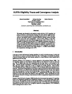
Figure 1: TBMin, the trailer backing mini-robot

2 Autonomous mini-robots We have designed and built two autonomous mini-robots in order to experiment with the SONNET paradigm. We describe the mini-robots now, because their limited computing power has imposed limitations in the design of their learning systems. One of the robots is called TBMin (Trailer Backing Mini-robot), the other is called PBMin (Pole Balancing Mini-robot). Most of the hardware controlling them is the same, but each robot has been designed for a speci c task, and the robots look dierent, as shown in Figures 1 and 2. Both robots have a chassis made from an inexpensive radio controlled car. The chassis of TBMin is made up of a car and a trailer. The body of the cars and most of the original electronics have been removed and replaced by boards speci cally designed at the Arti cial Intelligence, Robotics, and Vision Laboratory (AIR-VL) at the University of Minnesota. A 7.2 volt rechargeable battery is used to drive the car and the boards. The battery lasts approximately 15 minutes, and this limits the number of on-board learning trials we can perform. The boards are small (4 inches by 2 3/4 inches) and are stacked. The connections are made using wires plugged into connectors. We use three dierent boards: 2

Micro-computer board: The micro-computer board is built around a 68hc11 microcon-

troller. This board has 16k of ROM and 32k of RAM. The microcontroller we use is the most popular microcontroller for inexpensive robots. The limited size of the memory and the limited speed of the microcontroller have dictated many of the design choices in the implementation of the learning system. The board can be connected to a workstation through the asynchronous serial port to download programs and upload results; Motor board: This board is also built around a 68hc11 microcontroller. It has 16k of EPROM and a L293E dual-motor-driver chip. The motor board operates as a slave and communicates to the micro-computer board through a synchronous serial port (with a transfer rate of 62.5 kilobits/second). The motor board continuously runs a looping program that can run up to four dierent selectable programs; Interface board: This board synchronizes the synchronous serial communications between the micro-computer board and the motor board. This board has 8 LEDs used for debugging. The sensors used on the two robots are dierent, since each robot has a dierent task. All the information the robots are given to accomplish their tasks is obtained through the use of their sensors.

2.1 TBMin

The motor board on TBMin runs a steering controller and a light-tracker program. TBMin uses two inputs { the angle of the trailer to the target and the angle of the hitch (that is, the angle between the car and the trailer). The angle to the target is computed using a light-tracking head that follows a 100W light bulb. The light-tracking head is attached to a servo that is able to turn it up to 90 on either side. The motor board keeps the light tracking head pointed at the light bulb at all times. The micro-computer board reads the angle from the variable resistor in the servo using the analog port. The angle of the hitch is sensed using a variable resistor. As the trailer rotates to either side, the variable resistor turns, changing the resistance that is read by the micro-computer board. TBMin uses the original radio car controller and can read from the radio receiving board through the analog port. The radio board allows TBMin to be moved to initial positions using the radio controller rather than manually. TBMin also uses other sensors not needed by the neural network. To obtain smooth movements, the motor board keeps the car at a constant velocity, and prevents the steering motor from oversteering. This requires a pulse width modulator and a steering wheel position sensor. The 68hc11 uses the timing port to generate a pulse width modulation which keeps the car at a steady velocity. The steering position sensor is used to keep the steering motor from turning too far and damaging the motor. 3

Figure 2: PBMin, the pole balancing mini-robot

2.2 PBMin

Like TBMin, PBMin uses two sensor inputs. For PBMin, these inputs are the pole angle and the car position. The pole-angle sensor is a variable resistor attached to a common yard stick. The motor board reads the variable resistor through the analog port on the microcomputer board and returns 28 dierent angular positions for the pole. This is similar to the way in which TBMin obtains the angle of the hitch. The pole is limited to move up to approximately 12 in either direction. The car position is computed by dead reckoning, using a simple car position sensor we built. The position sensor uses two infrared sensors placed slightly less than half way around the wheel. A paper disk, half white and half black, is mounted on the wheel. As the car moves, the disk on the wheel rotates and the infrared sensors sense a dierent amount of infrared light, depending on whether the white part or the black part of the disk is presented to them. The motor board uses a look-up table and the previous sensor readings to compute in which direction the wheel has moved and increments or decrements the position. The wheel has a circumference of 6 inches so the car position can be measured to the nearest 1 1/2 inches. Figure 3 shows the pole-angle sensor and car-position sensor. 4

transmitter

IR modules

variable resister

(b)

pole disk

receiver

wheel (d) receiver

transmitter

(a)

shaft

(c) (e)

.

Figure 3: Sensors used for PBMin

3 Connectionist control-learning with self-organizing maps Connectionist control-learning systems have recently received much attention, and numerous papers and several books have been published on this topic in the previous ve years (e.g. [23], [19]). Most of these works, however, have concentrated on simulated systems and therefore have not had to deal with the ambiguities of actual robots. This section presents a class of connectionist control-learning networks together with the particular systems that were used on the two real mini-robots described above.

3.1 Terminology

Learning responses has generally been divided into supervised and unsupervised learning. In supervised learning an agent or function, often called the teacher, that can provide the desired output response for each input vector is required. Systems that do not make use of a teacher, then, are known as unsupervised learning systems. Within unsupervised learning, however, dierent levels of feedback may be available to the learning system. In many cases an evaluation of system output (either directly or through examination of the controlled system's new state) is immediately available. This allows learning to occur for each input vector and output response pair. We will here refer to learning with an immediate feedback system as guided learning and the feedback system itself as a critic [24]. We are concerned with learning in situations in which a less immediate response is available than in either the supervised or guided learning cases. In this paper we will examine 5

problems for which no feedback is available until the task that the system is to learn is completed. We will refer to these problems as terminal feedback problems. Further, we are interested in problems for which the terminal feedback is no more than a simple boolean value (a success or failure signal) returned by a binary, terminal evaluation function.

3.2 SONNET

Kohonen [12] has proposed a physiologically plausible method of cooperative and competitive organization for connectionist systems that allows them to self-organize around a set of input vectors. Several variants on Kohonen's Self-Organizing Topological Feature Maps (Kohonen Maps) have been suggested [10]. These have included networks which allow the learning of output values as well (e.g. for the control of physical systems, [20]). All of the variants involving output learning, however, have required the use of teachers or critics to provide desired responses or response evaluations (respectively) at each time step. While for many control-learning problems the existence of teachers or critics may be assumed, for other problems no such oracles may be available. For problems in which, at each time step, no acceptable response is known and no immediate feedback is possible but a terminal evaluation mechanism (success and/or failure signals) is available, Hougen [7] proposed the Self-Organizing Neural Network with Eligibility Traces (SONNET). One example of such a problem is the classic formulation of the \pole-balancing" problem, as given by [15]. The use of SONNET networks on this problem in simulation [7] and a restricted version of the problem for a real-world system [8] have been presented. SONNET works by combining the self-organizing capabilities of Kohonen Maps with the temporal sensitivity of eligibility traces. It should be recognized that the SONNET paradigm describes a class of connectionist learning systems, rather than a particular network.

3.3 Self-organizing maps

Unlike traditional layered neural networks which may have separate input, hidden, and output layers with dierent characteristics, Kohonen Maps have a single layer containing uniform neural elements. None-the-less, Kohonen Maps have an internal structure. The internal structure of a Kohonen Map is de ned by a topological ordering of the neurons that remains unaltered as the network learns. Most commonly, this topology is planar (two dimensional), but linear (one dimensional) networks have also been used in several instances (e.g. [7]), and higher dimensional networks are also possible. Three dimensional Kohonenbased networks have been used by Ritter, Martinetz, and Schulten (e.g. [20]) for the control of a robot arm. For the example below, a planar topology is used. For a planar topology, each neuron is uniquely numbered with a pair of integers which can be thought of as its coordinates in topology space. The existence of a network topology allows for the de nition of a \distance" function for the neurons based on their numbering. Typically, this is de ned as the Cartesian distance between coordinates in topology space. 6

1, 1

2, 1

3, 1

4, 1

5, 1

6, 1

7, 1

1, 1

1, 2

2, 2

3, 2

4, 2

5, 2

6, 2

7, 2

8, 2

1, 3

2, 3

3, 3

4, 3

5, 3

6, 3

7, 3

8, 3

1, 4

2, 4

3, 4

4, 4

5, 4

6, 4

7, 4

8, 4

1, 5

2, 5

3, 5

4, 5

5, 5

6, 5

7, 5

8, 5

1, 6

2, 6

3, 6

4, 6

5, 6

6, 6

7, 6

8, 6

1, 7

2, 7

3, 7

4, 7

5, 7

6, 7

7, 7

8, 7

1, 8

2, 8

3, 8

4, 8

5, 8

6, 8

7, 8

8, 8

topology but this is not necessary for some applications. For our example, the input space (like the topology) will have two dimensions, so each neuron will have two input weights. Often these weights are assigned random values initially, although for our purposes such a random distribution is not necessary. (In [8] the weights were assigned non-random initial values, for example.) What is necessary is that the weight values are changed as input is received in such a way that they come to re ect the input distribution. Each time a new input vector is given to the network the input weights are compared with the input and one neuron s is declared the \winner" and is selected according to the following equation:

9sfD(ws ; x)  D(wu ; x) j 8u 2 U; s 2 U g

(2) where each w is an input weight vector, x is the input vector, and D is a distance function de ned in the input space. If more than one neuron satis es equation 2, then one of these is selected by any arbitrary method. The weights of the neurons in the neighborhood Ns(t) of the selected neuron s are updated to match the input value even more closely according to the equation (

old old i 2 Ns(t) (3) = wwiold + (t)(x ? w ) if if i 62 Ns(t) i where  is a time dependent function which determines how much of the old weight value is retained. Typically, (t) starts near 1 and decreases with time.

w

new i

3.3.2 Cooperation

Although only a single neuron is selected as the winner, more than one unit may have its weights updated for each input that is received. All units within the neighborhood of the selected neuron are updated using equation 3 while the neurons outside the neighborhood remain unchanged. This inter-neuron \cooperation" is primarily responsible for the selforganizing properties of Kohonen Maps. It allows initially random networks to align their topology to the topology underlying the source of the input vectors appropriately and these partially ordered networks to distribute their neurons in the input space with a density matching that of the input distribution.

3.3.3 Self-organized output

Several authors (e.g. [20]) have adapted the self-organizing maps proposed by Kohonen to allow for the learning of output responses. To do this, these authors proposed that the network be given a set of output weights for each neuron in addition to the set of input weights. The required number of output weights per neuron is task-dependent and has ranged from one [7] to forty- ve [20]. For this example, we'll use one output value per neuron. 8

left

threshold

x right

cart-pole states

8 x 8 network

response

Figure 5: Mapping from cart-pole states to left-right output responses. Like the input weights, the output weights are typically given initial random values. With previous authors the output weights were updated using an equation similar to that used for the input weights (equation 3). This has required that a teacher be present to give the desired output response or that a critic be present to indicate the direction of the desired change in the weights. The absence of such a teacher or critic for some problems is the impetus for the use of the eligibility trace (see section 3.4). As with the input weights, the output responses are updated using inter-neural cooperation within some neighborhood of the selected neuron. Note that this neighborhood need not be the same as the neighborhood used for updating the input weights. In [8], a two-dimensional Kohonen-based map was used to learn to solve the polebalancing problem using two dimensions of the input space (the pole angle and cart position). This network can then be seen as learning a mapping from cart-pole states to output responses as shown in Figure 5.

9

3.4 The eligibility trace

The neurons which comprise animal brains are actually quite complex elements and only a few of their functions are approximated by today's arti cial neural networks. One function of biological neurons which has previously not been approximated in the more standard connectionist systems is what we refer to as the eligibility trace. It is known that many neurons become more amenable to change when they re (see, e.g. [11]). This plasticity reduces with time, but provides an opportunity for learning based on feedback received by the neuron after its activity. We have chosen to have this eligibility trace decay exponentially.

3.5 SONNET architectures

As the SONNET paradigm de nes a set of connectionist systems, many dierent particular architectures may be constructed that fall under this rubric and, in fact, several dierent architectures have been examined. Some of these are described below along with their respective strengths and weaknesses.

3.5.1 Independent linear networks

In [7], a network of four independent linear SONNET networks was applied to a simulation of the inverted pendulum problem. Four networks were chosen as the problem has a fourdimensional input space (see Section 5 below). Each network attempted to learn the correct response given only a single component of the input space vector and each network supplied its output response to a central function which selected the maximum response as the overall system response. This system used very few neural units and response time was extremely fast. Further, when a workable solution was arrived at, it was found in remarkably few trials. Unfortunately, the four independent networks lacked overall coordination and could not nd a solution in every case, depending on the initial random con guration of the weights.

3.5.2 Multi-dimensional networks

Overall system coordination is not a problem in multi-dimensional SONNET networks. A two dimensional SONNET network was applied by [8] to a restricted version of the polebalancing problem in which only the pole angle and cart position elements of the input vector were considered. The problem was restricted to a two-dimensional version because SONNET networks suer from memory and computational explosions with increasing dimensionality. In theory, this could be handled by special-purpose hardware (see Section 3.6) but if such is not available this explosion can prevent real-time response.

10

left

threshold

x

cart-pole states

right

one-dimensional networks

8 x 8 network

response

Figure 6: Mapping from cart-pole states to left-right output responses using separate input and output networks.

3.5.3 Separate input and output neural sets

An alternate mapping of cart-pole states to responses involving separate connectionist components for learning input and output is shown in Figure 6. While discussion up to this point has assumed that the network had a single set of neurons having both input and output weights, there is really no reason that this must be the case. Just as a network may have dierent updating functions for input and output weights, or dierent neighborhood sizes, etc., it is also possible to accommodate completely separate sets of neurons learning input and output. All that is needed for this variation is a method for moving from selected input neuron(s) to appropriate output neuron(s). A system of this variety is used in this paper for the control of TBMin using more neurons to learn the output space than have been used in previous papers discussing SONNET systems. These additional neurons allow for a ner resolution of output responses, but also reduce the system reaction time if they are used to partition the input space. Two independent linear networks (one for each term in the input vector) learn to partition the input space and a single two-dimensional network learns appropriate output responses as shown in Figure 6. On each time step one unit from each input network is selected 11

and the two numeric designators for these units are used to index into the two-dimensional network. This mapping between input and output networks is unchanging. This network con guration allows for quick response time (see Section 3.6.1) while retaining the interdimensional cooperative learning of a multi-dimensional network.

3.6 Use of SONNET in real-time, real-world systems

In theory, neural network systems should be ideally suited to implementation in time-critical domains. Since each neural element is a separate computing device, the massive parallelism inherent in the network, and the fact that each neuron need only compute a very simple function, should give extremely rapid response rates for the network. In practice, however, most neural networks are merely simulated on traditional sequential machines. This means that any simple computation must be calculated by the sequential processor once for each neuron in the network, potentially causing massive delays. For this reason it may be necessary to adapt the learning system calculations for real-time implementations. In this section we describe some of the modi cations that may be made to learning systems which must run in real time.

3.6.1 Indexed output neuron selection

As discussed above in 3.5.3, a single SONNET system may use two independent linear input networks to index into a single two-dimensional output network. If the two-dimensional network with a topology of 8 x 8 neurons were to be used for both input and output, then to select a winning neuron, all 64 neurons in the network would have to have their two input weights compared to the two-dimensional input vector. If, instead, two one-dimensional networks (of 8 neurons each) are used for partitioning the input space, only 16 neurons need to be referenced and each of these needs have but a single input weight. This results in a savings of 8 times in both computation time and memory requirements for neuron selection. As the output network grows larger, this savings will increase.

3.6.2 Approximated eligibility decay

While the eligibility decay is de ned to be a continuous exponential decay, a continual update is not necessary. Instead, it is sucient to update a particular neuron's eligibility level only when that neuron is selected. The key is to use a \half-life" of eligibility for this update. The half-life of eligibility is de ned to be the number of time steps it would take for any given original value of eligibility to fall approximately in half. For example, if the exponential decay rate is 0.9 then, after multiplying the current eligibility value by 0.9 for 6 time steps, one would get a value of approximately half of the original, so the half-life for this decay rate is 6. A record is kept of the last update time for each neuron, and when a neuron is selected an approximation of the decay that should have taken place since the last ring is computed using the following pair of equations: 12

(t ? n) AE (t) = E(n=L )2

E (t) = AE (t) ? AE (t) (2nLmod L) where E (t) is the eligibility, AE (t) is the approximate eligibility, n is the number of time steps since the last update, and L is the half-life for eligibility. Use of this approximation means that only one neuron need have its eligibility values updated on any given time step, as only a single output neuron is selected. Since the number of neurons updated per time step remains constant (at one), regardless of network size, this adaptation (like indexed output neuron selection) becomes even more useful as network size increases.

3.7 SONNARR

The connectionist system we propose for learning on the trailer-backing mini-robot is SONNARR (Self-Organizing Neural Network Applied to Real Robots). Whereas SONNET refers to a class of connectionist networks, SONNARR refers to the particular network used in this application. It is based on the SONNET paradigm, but has several unique adaptations to allow it to work under the constraints imposed by the micro-computer board. First, SONNARR uses integer values for all computations. While the 68hc11 microcontroller is able to process oating point values, doing so is simply too computationally expensive to allow for any reasonable number of computations to be performed in real time. Second, SONNARR uses the seperate input and output networks, as described in Section 3.5.3. For the pole-balancing task response time is absolutely critical. For an 8 x 8 network handling both input and output learning, the total response time for pole-balancing would be an estimated 20 cycles per second. With two seperate one dimensional networks (of 8 neurons each) learning the input space, the system is able to respond more than twice that fast. Third, SONNARR uses the approximated eligibility decay, as described in Section 3.6.2. An operation pair consisting of a single multiplication and division operation for each neuron is thereby replaced by a more complex operation (of roughly seven computations equal in computational expense to a single multiplication operation) which need only be calculated for a single neuron. Since SONNARR has 64 output neurons, this approximation takes about one ninth the time that the straightforward exponential decay would have taken.

4 Experimental results This section describes our experimental results, obtained both in simulation and with the two mini-robots described earlier. In our experiments we were mainly interested in answering the following questions: 13

 Is the SONNET paradigm suciently general to be applicable to learning very dierent

tasks? We selected the two tasks of backing up a trailer and balancing a pole to test the generality of the paradigm. Both robots run networks constructed on the SONNET model. SONNARR, used with TBMin, is described above. With PBMin, a similar network (with the same name as the robot itself) was used. It is fully detailed in [8]. Hardware-speci c code to handle the dierent sensors on each robot was used as well as a velocity controller for backing the trailer.

 Can the SONNET paradigm be used in real-time applications with limited computing

power? Our mini-robots have limited memory and limited processing power so the approach we use must require no more computation power that what we have available.

 How well can the real robots learn the desired task? For TBmin the percentage of

successes in backing was measured. For PBMin, the the period of time the system can balance the pole after learning compared to the time it can balance the pole without any learning was considered.  How fast can the real robots learn the desired task? The limited battery life imposes serious limitations on the number of training runs and any method that requires more that 40-50 training runs using the actual robot is impractical. Even though other learning approaches might produce good results in simulation, any method that requires a very long training phase has to be ruled out, unless we can use the learning done in simulation to speed up the learning on the real robots. This brings up the next research question.  How useful is it to start learning in simulation and then complete the learning on the real robots? Will the real robots start their learning with useful knowledge, or do they have to unlearn what the simulation has produced and to start learning again? Since it is likely that the results obtained in simulation will depend on the accuracy of the model of the physical system used in simulation, there is one more important question.  How important is to use an accurate simulation model when performing learning in simulation? In our experiments we use a quite good model of the physical system for backing up the trailer, but a much more crude model of the physical system for balancing the pole. Factors such as the wind resistance of the pole and the slippage of the wheels on the oor are not modeled at all, yet they seem to be important for the real robot to succeed at doing the task. Despite the fact that we do not estimate the pole-angle velocity and the car velocity, our real robot succeeds at balancing the pole for over 350 time steps (see [8]).

4.1 Trailer backing

TBMin has a 2m2 area to back up the trailer. Failure occurs when the angle of the hitch exceeds 45 or when the angle to the target reaches approximatively 90 or when the rear 14

2 1/4 in.

Hitch Angle Wheel Angle

Goal 8 1/4 in.

Goal Angle

6 1/4 in.

Figure 7: The trailer-backing problem of the trailer reaches the target but the value of the trailer and/or hitch angles are greater than 20. Success occurs when the rear of the trailer reaches the target and the angle of the trailer and the hitch are each less than 20. The learning system gets one signal for success and a dierent signal for failure, allowing it to dierentiate between these cases. On each time step the learning system is given the current values of the trailer and hitch angles and, if applicable, a failure or success signal. The network response is thresholded and values less than zero are used as hard left control signals, while values equal to or greater than zero are used as hard rights by TBMin. In this way, the system is given bang-bang control, which corresponds to the control allowed in the pole-balancer problem which we previously studied. Note that the output values would not have to be thresholded and the system could learn smoother control, if appropriate hardware were utilized. We plan to examine this possibility in the future. The learning is performed using several training runs conducted in simulation. For the rst 100 trials the trailer is placed ve scale feet from the target and at random angles from ?60 to 60 with the cab at an angle of ?30 to 30 with the trailer. This period of training corresponds to the \observation trials" used by [7]. The system is then started on a series of training runs of increasing diculty. Initially the trailer was placed at short distances from the target and at small angles to it and the cab was placed at small angles to the trailer. Incremental steps of diculty were added until the trailer was placed at a distance of 6 scale feet from the target and at an angle of ?45 to 45 and the hitch angle was set from ?20 to 20 . These increasingly dicult \lessons" are consistent with the training schemes used by other authors (e.g. [17]). After a total of 1000 training trials, the learned responses were tested in simulation and on TBMin. A sample simulation run after training is depicted in Figures 8, 9, and 10. The angle of the trailer and of the hitch are depicted graphically for a sample simulation run in Figure 11 and for a sample run on TBMin in Figure 12. 15

Figure 8: TBMin, initial state

Figure 9: TBMin, a run

Figure 10: TBMin, nal state 16

Figure 11: TBMin, simulation log

Figure 12: TBMin, real log

17

12° θ

x -4.0m

4.0m

Figure 13: The Pole-balancing problem

5 Pole balancing Pole-balancing grew out of a classic dynamics problem (see e.g. [3], [18]) and is now a wellstudied control-learning problem (see 7). For the control-learning form of the problem the system must learn to keep a long rod or pole, hinged to a cart and free to fall in a plane, in a roughly vertical orientation by applying forces to the cart. If the pole passes a certain value from the vertical (de ned to be 12 by most authors and we have followed suit), or the cart goes beyond a certain xed distance from its starting point, a failure signal is generated. Unlike the trailer-backing system, no success signal is ever generated in the pole-balancer. In our simulations and implementations on real robots, we have used bang-bang control for the application of the force to the cart, as this is the traditional formulation of the problem. The fact that the output weights for SONNET networks are scalar valued rather than binary, however, means that a solution involving more nesse could be learned with SONNET systems.

6 Evaluation of SONNET The learning method we have described satis es the requirements stated by [14] for a robot learning method. Our experiments show that the method is quite immune to noise in the sensor data, converges quickly, is incremental, is tractable in real-time, and it is grounded.

7 Related work The pole-balancing problem has been a subject of study by researchers in the area of controllearning for over thirty years now. Such now-classic approaches as ADALINE [25] and BOXES [15] were applied to the pole-balancing problem when they were still new. A great many later researchers have also studied this problem. For an extensive, though somewhat faulty, list of references see Geva and Sitte [5]. 18

This problem has proven to be of reasonable diculty for supervised-learning systems (e.g. [25], [6]), more dicult for guided-learning systems (e.g. [4]), and extremely dicult for terminal-evaluation systems (e.g. [1]). The trailer-backing problem has not been studied as long or as extensively as the polebalancing problem, but it too is becoming widely studied. Approaches such as the Cerebellar Model Articulated Controller (CMAC) [21], adaptive fuzzy systems [13], backpropagation through time [16, 17], and \fuzzy BOXES" [26] have all been applied to this problem.

7.1 Comparison with related work

While many researchers have studied the pole-balancing or trailer-backing problems (or both, e.g. [26]), it is very dicult to directly compare results across many of these systems and we nd it dicult to directly compare our results with theirs. Perhaps the most obvious dierence between our studies and those of most other authors writing on either problem, is that our learning systems were implemented on real robots, whereas theirs were restricted to simulated systems. Restricting their attention to simulated systems for control has freed many researchers from having to deal with unpleasantries such as noisy input data and variable amounts of wheel slippage, although some researchers have tried to model these types of eects in simulation (e.g. [22]). The use of simulation has also allowed other researchers to include many more learning trials in their training runs and to use learning systems with much greater memory and computational demands. For these reasons, results such as successful pole-balancing for 2.8 hours of simulated real time [2] should not be directly compared with results obtained in real-world robotic systems. We are aware of no other research involving truck-backing using real robots and the only previous works of which we are aware that discuss learning to solve the pole-balancing problem using real robotic systems are Jervis and Fallside [9] and Hougen, et al. [8]. As the physical parameters the two systems are quite dierent, direct comparison of results is not possible. Neither is it possible to run our learning systems in simulation and directly compare simulation results with those of most other authors, as various authors have de ned the problem dierently. If only the simulated physical systems were dierently de ned (e.g. longer or shorter trailer in the trailer-backing problem or heavier or lighter cart in the pole-balancing problem), then a few constants could be adjusted and comparable results obtained. The greater dierences between researchers studying these problems, however, is their formulation of the problem with regard to information provided to the learning systems, either during the learning phase (supervised vs. guided vs. unguided) or hardcoded into the learning system (for example, the de nition of the boundaries of the boxes in the BOXES system). In Hougen[7], for example, only a single truly comparable system was found against which results for the proposed system could be pro tably measured. A standard for pole-balancing simulations (primarily following the classic parameters of Michie and Chambers [15]) and evaluations was recently proposed by Geva and Sitte [5]. Unfortunately, these authors seem to have overlooked the importance of provided information 19

in comparing systems. They do not seem to realize that the problem, as formulated in the classic BOXES paper, provides no opportunity for systems to learn criteria that they deem important for evaluating performance, for example. To our knowledge, no such set of standards has yet been proposed for the trailer-backing problem, although a carefully determined set of standards might well prove useful. Another major dierence is the input variables that the system is to learn from. In most versions of the pole-balancing problem, four input values are passed to the system (cart position, cart velocity, pole angle, and pole angular-velocity). In Hougen et al. [8], only cart position and pole angle are used. A similar discrepancy between common practice and our choice of input vectors is to be found with the SONNARR system presented here. Whereas most truck-backing systems include such variables as the x and y position of the rear of the trailer in Cartesian space, we do not. This is primarily because our system is designed to operate in the real world. Whereas the x and y coordinates are easily determined in simulation (in fact, are used in the mathematical model of the simulation), they are quite dicult for an autonomous robot to acquire. Instead, we use only the angle of the trailer to the target and of the hitch. There are also relatively minor discrepancies which have not yet been covered (such as bang-bang vs. multiple discrete divisions vs. continuous control of steering). All of the dierences taken in combination make it clear that simple comparison of success rates between SONNARR and other learning systems for trailer-backing are of no value.

8 Conclusions We have described a paradigm for learning simple tasks for real robots and we have presented experimental evidence to support our proposed approach. SONNET has proven useful paradigm for the development of a rapid learning system for real robotic systems (see the results for PBMin presented in [8]), as well as the creation of a simulation to real-world application system such as SONNARR, presented herein. The paradigm is rich with possibilities for further study, including novel network architectures and hybridization with other systems (such as self-learning critics).

9 Acknowledgements This research was conducted at the Arti cial-Intelligence, Robotics, and Vision Laboratory at the University of Minnesota. We would like to thank Chris Smith and all the other members of the AIR-VL for their help, moral support, and patience with us.

References [1] Charles W. Anderson. Learning to control an inverted pendulum using neural networks. IEEE Control Systems Magazine, 9(3):31{37, 1989. 20

[2] A. Barto, R. Sutton, and C. Anderson. Neuronlike adaptive elements that can solve dif cult learning control problems. IEEE Transactions on Systems, Man, and Cybernetics, SMC-13:834{846, 1983. [3] R. Cannon. Dynamics of Physical Systems. McGraw-Hill, New York, 1967. [4] M. Connell and P. Utgo. Learning to control a dynamic physical system. In Proc. Nat'l Conf. on Arti cial Intelligence, volume 2, pages 456{460, Seattle, 1987. [5] Shlomo Geva and Joaquin Sitte. A cartpole experiment benchmark for trainable controllers. IEEE Control Systems Magazine, pages 40{51, October 1993. [6] A. Guez and J. Selinsky. A trainable neuromorphic controller. Journal of Robotic Systems, 5(4):363{388, 1988. [7] Dean F. Hougen. Use of an eligibility trace to self-organize output. In Science of Arti cial Neural Networks II, Proceedings SPIE, volume 1966, pages 436{447, 1993. [8] Dean F. Hougen, John Fischer, and Deva Johnam. A neural network pole balancer that learns and operates on a real robot in real time. In Proceedings of the MLC-COLT Workshop on Robot Learning, pages 73{80, 1994. [9] T. Jervis and F. Fallside. Pole balancing on a real rig using a reinforcement learning controller. Technical Report CUED/F-INFENG/TR 115, Cambridge University Engineering Department, Cambridge, England, 1992. [10] J. A. Kangas, T. K. Kohonen, and J. T. Laaksonen. Variants of self-organizing maps. IEEE Transactions on Neural Networks, pages 93{99, 1990. [11] A. Klopf. Brain function and adaptive systems { a heterostatic theory. In Proceedings of the International Conference on Systems, Man, and Cybernetics, 1974. [12] T. K. Kohonen. Self-organizing and associative memory. Springer-Verlag, Berlin, 3rd edition, 1989. [13] Seong-Gon Kong and Bart Kosko. Adaptive fuzzy systems for backing up a truck-andtrailer. IEEE Transactions on Neural Networks, 3(2):211{223, March 1992. [14] Sridhar Mahadevan and Jonathan Connell. Automatic programming of behavior-based robots using reinforcement learning. AI, 55:311{365, 1992. [15] D. Michie and R. Chambers. Boxes: an experiment in adaptive control. In E. Dale and D. Michie, editors, Machine Intelligence. Oliver and Boyd, Edinburgh, 1968. [16] D. Nguyen and B. Widrow. The truck backer-upper: an example of self-learning in neural networks. In Proceedings of the International Joint Conference on Neural Networks, volume II, pages 357{363. Erlbaum, 1989. 21

[17] D. Nguyen and B. Widrow. Neural networks for self-learning control systems. IEEE Control Systems Magazine, 10(3):18{23, 1990. [18] K. Ogata. System Dynamics. Prentice-Hall, Englewood Clis, New Jersey, 1978. [19] H. Ritter, T. Martinetz, and K. Schulten. Neural computation and self-organizing maps: an introduction. Addison-Wesley, Reading, MA, 1992. [20] H. Ritter and K. Schulten. Extending Kohonen's self-organizing mapping algorithm to learn balistic movements. In R. Eckmiller and C. von der Malsberg, editors, Neural Computers, volume F41, pages 393{406. Springer, Heidelberg, 1987. [21] Robert O. Shelton and James K. Peterson. Controlling a truck with an adaptive critic CMAC design. Simulation, 58(5):319{326, 1992. [22] T. Troudet and W. Merrill. Neuromorphic learning of continuous-valued mappings from noise-corrupted data. IEEE Transactions on Neural Networks, 2(2):294{301, 1991. [23] III W. Thomas Miller, Richard S. Sutton, and Paul J. Werbos. Neural Networks for Control. MIT Press, Cambridge, MA, 1990. [24] Bernard Widrow, Narendra K. Gupta, and Sidhartha Maitra. Punish/reward: learning with a critic in adaptive threshold systems. IEEE Transactions on Systems, Man, and Cybernetics, SMC-3(5):455{465, 1972. [25] Bernard Widrow and Fred W. Smith. Pattern-recognizing control systems. In COINS (Computer and Information Sciences Symposium), pages 288{317, Washington, DC, 1964. [26] N. Woodcock, N. J. Hallam, and P. D.Picton. Fuzzy BOXES as an alternative to neural networks for dicult control problems. Arti cial Inteligence in Engineering, pages 903{ 919.

22