learning. We studied in our previous work [1], [2] the game Connect Four (Connect-4, Sec. ...... It is surprising that the system breaks down completely for λ ⥠0.9.
Temporal Difference Learning with Eligibility Traces for the Game Connect Four Markus Thill, Samineh Bagheri, Patrick Koch and Wolfgang Konen Department of Computer Science Cologne University of Applied Sciences 51643 Gummersbach, Germany Abstract Systems that learn to play board games are often trained by self-play on the basis of temporal difference (TD) learning. Successful examples include Tesauro’s well known TD-Gammon and Lucas’ Othello agent. For other board games of moderate complexity like Connect Four, we found in previous work that a successful system requires a very rich initial feature set with more than half a million of weights and several millions of training games. In this work we study the benefits of eligibility traces added to this system. To the best of our knowledge, eligibility traces have not been used before for such a large system. Different versions of eligibility traces (standard, resetting, and replacing traces) are compared. We show that eligibility traces speed up the learning by a factor of two and that they increase the asymptotic playing strength.
I.
I NTRODUCTION
Games are an ideal testbed for complex learning tasks. They can be repeated numerous times in a controlled game environment. The task of the learning agent is to collect the necessary information from multiple games to form a good strategy. The problem in board games is that the reward is usually only given at the end of the game and it is often difficult to assign a credit to each action (move), when the final reward lies in the future (credit-assignment problem). One way to assess this problem is temporal difference learning (TDL), a special form of reinforcement learning. We studied in our previous work [1], [2] the game Connect Four (Connect-4, Sec. I-B) as an example. We showed that a combination of TDL with a specific feature set (the so-called n-tuple system, Sec. II-A) can successfully learn that game. A key to success is a rather big feature space resulting in a system with several millions of weights. Not surprisingly, our first solution had the drawback that the training of the agent requested a huge number (several millions) of training games as well. The final success rate was with 90% quite high, but there is still room for improvement with respect to the missing 10%. In this paper we investigate new strategies for speeding up the learning and strengthening the final success rate. These strategies are: A) Eligibility traces: This is a well-known strategy in TDL which, in the case of sparse input vectors, allows more weights to participate in learning during a specific episode. Eligibility traces propagate rewards back to earlier visited states, diminished by a discount factor for each step back. In our previous work we were quite reluctant to use eligibility traces because a na¨ıve implementation would add several million trace parameters to the system (corresponding to the number of weights). We present in this work a more efficient implementation circumventing this problem. Several variants of eligibility traces are compared. B) Larger n-tuple systems: If an efficient implementation is available, it is natural to ask whether a larger feature space would increase either learning speed, final accuracy, or both. Preprint version of: Markus Thill, Samineh Bagheri, Patrick Koch and Wolfgang Konen, ”Temporal Difference Learning with Eligibility Traces for the Game Connect Four”, in: M. Preuss, G. Rudolph (Eds.), CIG’2014, International Conference on Computational Intelligence in c IEEE, http://ieeexplore.ieee.org/xpl/mostRecentIssue.jsp?punumber=6919811. Games, Dortmund, pp. 84 – 91, 2014.
2 1
1
2
1
1
0 3
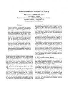
Fig. 1. Typical Connect-4 position, created during a match of a temporal difference learning agent (Yellow) against a perfect playing Minimax agent (Red). Minimax is under zugzwang and will loose the game, however, the defeat could be delayed as far as possible. Additionally, this figure shows an example 4-tuple state and its mirrored equivalent (Sec. II-A).
A. Related Work Temporal Difference Learning (TDL) was successfully applied for playing checkers by Samuel [3] and became popular with the Backgammon agent proposed by Tesauro [4], [5]. There have been various follow-ups of Tesauro’s TD-Gammon for other games, e.g., TicTacToe [6], Go [7] and Connect-4 [8], but mostly with discouraging results. Recent work in this field mainly includes extensions of the original TDL algorithm, such as Coevolutionary TDL [9], [10] or n-tuple systems [11]. Also van Seijen and Sutton [12] proposed a new online version of TD(λ) which outperformed the classical TD(λ) algorithm on two small tasks. Runarsson and Lucas [13] study preference learning in games as an interesting alternative to TDL. Thill et al. [1] established a TDL agent for the game Connect-4 solely trained by self-play. Although Connect-4 is solvable by computer programs [14], [15], the game remains difficult to learn with self-playing agents. For this reason most trained players for Connect-4, e.g., Schneider et al. [16], Curran and O’Riordan [17], and Stenmark [18], do not use perfect-playing agents as opponents. A pre-calculated Minimax agent that finds the perfect next move can help to give better insights into the real playing strength of TDL agents for Connect-4. With Minimax as opponent, Thill et al. [1] could reliably measure the agents’ strength and established that the time-to-learn (80% success rate, Sec. III-B) was 1.5 million games. Based on the work of [1], Bagheri et al. [2] improved the time-to-learn by a factor of 3 to 0.5 million games. This was achieved by adapting the learning rates of the algorithm using methods like Temporal Coherence Learning [19] or Incremental Delta-Bar Delta [20]. However, in all of the algorithms above, the rewards are only propagated one step back to earlier states in each episode. This can result in slow learning and high computing times. A possible solution to this problem are eligibility traces introduced in the TD(λ) algorithm [21] and further developed by Singh and Sutton [22]. TD(λ) combined with self-play has been successfully proposed for the card game hearts [23], Go [24], give-away checkers [25], and Backgammon [26]. To the best of our knowledge, no results have been reported for the game Connect-4, although Stenmark briefly describes eligibility traces in [18]. Larger systems with eligibility traces are not found very often in the literature. An remarkable exception is the work of Geramifard et al. [27] extending a special TD algorithm (iLSTD) with eligibility traces for a system with n=10 000 traces. To the best of our knowledge, no results were reported so far for systems with more than a million of traces, as they occur in our task here.
B. Connect-4 Connect-4 is a popular board game for two players (typically Yellow and Red) played on a board with seven columns and six rows. One main characteristic of the game is the vertical arrangement of the board: Starting with Yellow, both players in turn drop one of their pieces into one of the seven columns (slots). Due to the gravity-rule, the pieces then fall down to the lowest free position of the respective slot. A slot containing six pieces is considered as full and reduces the number of possible moves for both players by one (initially, seven moves are possible). The goal of both opponents is to create a line of four pieces with their color, either horizontally, vertically or, diagonally. The player who can achieve this first, wins the game. After 42 plys1 , all columns will be completely filled and the match ends with a tie, if none of the opponents was able to create a line of four own pieces. Connect-4 has a state space complexity of around 4.5 · 1012 different positions [28]; solving the game is still a non-trivial task: typically sophisticated tree-based algorithms are necessary in order to solve Connect-4 within a few days. Nevertheless, a solution was found independently by Allen [15] and Allis [14] in 1988. Their work proved that – assuming perfect play of both opponents – the starting player (Yellow) can always win by placing her first piece in the center slot. Red on the other hand, can delay her defeat as far as possible and force Yellow to use all her pieces. An example position is shown in Fig. 1 where Red will loose after 2 plys. II.
M ETHODS
A. N-tuple Systems Even though n-tuple systems were already introduced by Bledsoe and Browning in 1959 for character recognition purposes [29], their application to board games is rather new. Recently, Lucas [11] introduced an n-tuple architecture that can be used for approximating position value functions in board games like Othello.2 An n-tuple is defined as a sequence of length n of so-called sampling points Tν = (τν0 , τν1 , . . . , τνn−1 ), addressing a subset of all possible board cells. Connect-4 consists of 7 × 6 = 42 cells in total, so we code the cells with τνj ∈ {0, . . . , 41}. N-tuple systems can be viewed as a set of n-tuples and corresponding look-up tables, that form a linear position value function V (st ). Depending on the current occupation of cell τνj and the cell beneath, its current state can assume a value st [τνj ] ∈ {0, . . . , P − 1}. We distinguish P = 4 states: 0 = empty and not reachable, 1 = Yellow, 2 = Red, 3 = empty and reachable. By reachable we mean an empty cell that can be occupied in the next move. The reason behind this is that it makes a difference whether e. g. three yellow pieces in a row have a reachable empty cell adjacent to them (a direct threat for Red) or a non-reachable cell (indirect threat) [1]. With P = 4 possible values per sampling point, every n-tuple (of length n) can have P n different states. Each n-tuple state is mapped to an unique index value kν ∈ {0, . . . , P n − 1} with i = kν =
n−1 X
st [τνj ]P j .
(1)
j=0
For every n-tuple state, the generated index can be used to address a weight wi,ν,t in a look-up table LU Tν associated with n-tuple Tv . We maintain two look-up tables per n-tuple, one for each player. Generally speaking, the individual LUTs can be considered as parameter vectors w ~ v,t that will be adjusted in every time step t during the training. One improvement when using n-tuple systems is the utilization of board symmetries, which are very common in many board games. In Connect-4, the mirroring of the board along the central column leads again to an equivalent position. With this in mind, we can calculate an additional index value k ν of the mirrored Connect-4 board. The 1
A ply is a single move of one player, Yellow or Red. This n-tuple approach works in a way similar to the kernel trick used in support vector machines (SVM): The low dimensional board is projected into a high-dimensional feature space by the n-tuple indexing process [11]. 2
individual weights of w ~ v,t are then activated according to a state-dependent input vector ~xν (st ), generated as follows: (
xi,ν (st ) =
1, 0,
�
if i ∈ kν , k ν . otherwise
(2)
Fig. 1 shows an example board position with a 4-tuple and its mirrored equivalent. Assuming that we follow the ntuple on the left hand side from its lowest sampling point to its highest, the corresponding index values are calculated as k = 1 · 40 + 2 · 41 + 1 · 42 + 1 · 43 = 89. Likewise, the mirrored n-tuple has k = 147. For a given board position at time step t, the output for each n-tuple is generated by calculating the dot product w ~ ν,t · ~xν (st ). Since we typically have a system of m n-tuples Tν with ν = 1, . . . , m, the overall output of the n-tuple network can be formulated as a linear function n
�
f w ~ t , ~x(st ) =
m PX −1 X
wi,ν,t · xi,ν (st )
(3)
ν=1 i=0
where w ~ ν,t and ~xν (st ) are considered here as sub-vectors, contained in two big vectors w ~ t and ~x(st ), respectively. All weights in w ~ t are updated according to the TDL update rule (Sec. II-B). Our standard n-tuple system consists of 2 × 70 × 8-tuples 3 and it has 9 175 000 adressable weights. Due to many non-realizable n-tuple states,4 the number of weights that get activated during training is substantially lower. Our standard n-tuple system has only about 7% realizable states, i. e. only 600 000 − 700 000 of all addressable weights are ever activated during training.5 Note that the input vector ~x(st ) for a given board position is even more sparse: Each of the 70 n-tuples has only 2 states activated, thus only 0.02% (≈ 2 · 70/650 000) of all realizable states will carry a 1. B. Temporal Difference Learning The goal of almost all game-playing agents is to learn to predict the ideal value function. Ideally, at a given time step t, a state value function V (st ) should indicate how desirable a state st ∈ S is for the agent, where S is the set of all states. Typically, the value function maps a state to a real value. Temporal Difference Learning (TDL) can be one approach for learning such a value function, by viewing the game as a reinforcement learning (RL) problem: An initially inexperienced agent plays a sequence of games against itself. When the game terminates in a final state R(sf ), the environment returns a reward R(sf ) ∈ {−1.0, 0.0, 1.0} for {Red-win, Draw, Yellow-win}. Because rewards are only given in terminal states, the purpose of V (st ) is to estimate the expected future reward for all other states. We choose this function to have the form ��
V (st ) = y(w ~ t , ~x(st )) = σ f w ~ t , ~x(st )
(4)
with σ = tanh, the parameter vector w ~ t (containing adjustable weights), a state-dependent input vector ~x and a function f . In our case, f is given by Eq. (3) (simply the dot product of w ~ t and ~x). TDL attempts to learn the parameter vector w ~ t by minimizing the mean-squared approximation error (weighted proportional to state frequency). As the ideal value function is unknown, TDL approximates the error of a state at a given time step t with a bootstrapping approach, by selecting the best successor move st+1 and simply calculating temporal differences according to [21]: δt = R(st+1 ) + γV (st+1 ) − V (st ),
(5)
where R(st+1 ) is the reward for the successor move and V (st ) is the current approximation of the value function.6 Usually δt is referred to as the temporal difference (TD) error signal, which is used to train the weight vector w ~t 3
good compromise between computation time and accuracy Non-realizable states occur for n-tuples with one cell beneath the other: The upper cell cannot be in state 1,2, or 3 if the lower cell is in state 0 or 3. 5 The same ratio holds for bigger n-tuple systems: An n-tuple system with 2 × 150 × 8-tuples has about 1 300 000 − 1 500 000 active weights. 6 V (st+1 ) is set to 0 for a final state st+1 . 4
according to the following update rule: wi,t+1 = wi,t + αδt ∇wi V (st ) 2
(6)
�
= wi,t + α 1 − V (st ) δt xi .
This weight update aims at moving the current prediction closer to the prediction of the successor state. The complete TDL algorithm is summarized in Algorithm 1. Further details on TDL in strategic board games can be found in [30]. C. TD(λ) and Eligibility Traces Most board games such as Connect-4 have in common, that rewards – given by the environment – are delayed. Generally, a whole sequence of actions is necessary to reach a state in which the final reward is given. As mentioned before, temporal difference methods can be useful for solving reinforcement learning problems with such delayed rewards. However, even though simple (one-step) TD methods are able to learn value functions that predict the expected future reward, they still have to deal with some delay in the updates of their value functions: TD methods estimate in a bootstrapping process the temporal difference error for a state st based on the current prediction of the successive state rather than on the final outcome (reward). This means that a reward given at the end of a sequence of actions is only used to adjust the last prediction of the episode and predictions before the last one will not be updated. Thus, one-step TD methods can result in a slow learning process. As a simple example, assume that an agent constantly follows a policy π . This policy may result in an episode with T time steps and a final reward rT . After completing the first episode, the agent receives a reward from the environment and updates the value for V (sT −1 ). During the second episode, the value V (sT −2 ) can be adjusted and so forth. In this example, T − 1 repeated episodes would be required, until a delayed reward finally affects V (s0 ). In the case of large T , this can be problematic and can result in a slow convergence of the learning process. But if the agent constantly follows his policy π anyhow, then the predicted values of all states can directly be set to the final reward, i. e. V (s0 ) = V (s1 ) = · · · = V (sT ) = rT . In order to use training samples more efficiently, it is thus convenient to assign some credit to the preceding states {st−1 , st−2 , . . .} as well, when updating the value function for the current state st , since these preceding states led to the agent’s current situation. Monte Carlo methods follow this general idea, by approaching the backups in a rather different way than simple TD methods [31]: Instead of updating the value function based on temporal differences of predictions, Monte Carlo algorithms first complete a whole episode of length T and then update the value of each state visited during this specific episode. In contrast to TD methods, the backups for st are not based on any predictions, only the final reward rT provided by the environment is used: the values for all visited states of the corresponding episode are updated to that rT . However, one main disadvantage of Monte Carlo algorithms is, that the actual learning step cannot be performed until the final outcome of the episode is known. The TD(λ) algorithm, introduced by Sutton [21], synthesizes the plain TD method with the Monte Carlo method by combining the advantages of both approaches. The new ingredient in TD(λ) is the so called eligibility trace vector, containing a decaying trace ~et = (ei,t )T for each weight wi [21]: ~et =
t X
(λγ)t−k ∇w~ V (sk )
k=0
= λγ~et−1 + ∇w~ V (st ),
(7)
~e0 = ∇w~ V (s0 ),
with a trace decay parameter λ and a discount factor γ (we assume γ = 1 throughout this paper), which decay (or discount) the individual traces ei by the factor λγ in every time step. Thus, the effect of future events on the corresponding weights wi exponentially decreases over time. By choosing λ in a range of 0 ≤ λ ≤ 1, it is possible to shift seamlessly between the class of simple one-step TD methods (λ = 0) and Monte Carlo methods (λ = 1) [31]. Replacing traces: The definition of the conventional eligibility traces in Eq. (7) implies, that each trace accumulates
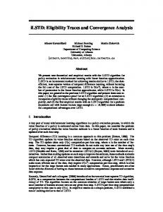
Fig. 2. Schematic view of different eligibility trace variants: Line a shows the situation without elig. traces, a weight is activated only at isolated time points. The dotted vertical line represents a random move. Line b shows the eligibility trace with reset on random move. Line c shows replacing traces, this time without reset on random move.
a value ∆ei = ∇wi V (st ) in every time step t if the corresponding weight is activated. In certain cases, this behavior may be undesirable, since specific states can be visited many times during one episode. As a result, the according traces build up to comparatively large values and future TD errors give higher credit to frequently visited states, which could negatively affect the overall learning process. Although a board state in Connect-4 is not revisited during an episode, a certain feature state (as it is introduced for example with the n-tuple states of Sec. II-A) might be active in many time steps of an episode. Thus, certain traces are addressed repeatedly. Replacing eligibility traces as proposed by Singh & Sutton [32] depict an approach to overcome this potential problem related to conventional eligibility traces. The main idea behind replacing traces is to replace a trace with ei = ∇wi V (st ) each time the corresponding weight is activated, instead of accumulating its value. As before, the traces of non-active weights gradually decay over time and make the weights less sensitive to future events. In this work, we will investigate both approaches, conventional and replacing eligibility traces. An example illustrating both types of traces is given in Fig. 2. Resetting traces: The TD(λ) algorithm usually requires a certain degree of exploration during the learning process, thus, the execution of random moves from time to time – ignoring the current policy. When performing random moves, the value V (st+1 ) of the resulting state st+1 is most likely not a good predictor for V (st ). The weight update based on V (st ) is normally skipped in this case. This also raises the question how to handle exploratory actions regarding the eligibility traces. We will consider two options: 1) Simply resetting all trace vectors and 2) leaving the traces unchanged although a random move occured. Both options may diminish the anticipated effect of eligibility traces significantly, if higher exploration rates are used (which is not the case in our experiments). Implementation: The number of eligibility traces equals the number of addressable weights (over 9 millions in our standard n-tuple system) which seems prohibitively high at first sight. We realized however that in our application Connect-4 the input vector ~x(st ) is very sparse and consequently the trace vector ~et is sparse as well. It can be shown 7 that during one game (episode) on average only 1 800 individual traces are non-zero for our standard n-tuple system (about 3 600 in the case TCL-M). After each episode the trace vector is reset again. Consequently, the additional resources needed to implement eligibility traces can be reduced to a reasonable amount: we implement the trace vector using a sparse representation (self-balanced binary tree, treemap). This reduces the memory requirements by a factor of 5 000: Instead of 9 million addressable traces we realize in each episode only the active traces which are 1 800 on average. The incremental TD(λ) algorithm for two-player board games, including the options for replacing (REP ) and resetting (RES ) traces, is listed as pseudo code in Algorithm 1. 7
An upper bound for the number of traces per game is the number of moves (42) times the number of n-tuples (70) times 2 (mirror states) = 5 880. The actual number is smaller since not every move activates a new state in each n-tuple. We found that on average around 1 800 individual traces are produced per game (for the setting TCL [et]), which is a comparatively small number.
Algorithm 1 Incremental T D(λ) algorithm for board games based on [30]. Prior to the first game, the weight vector w ~ is initialized with random values. Then the following algorithm is executed for each complete board game. During self-play, the player p switches between +1 (Yellow) and −1 (Red). In our experiments we use γ = 1 throughout. Set REP = true, if using replacing traces Set RES = true, if resetting elig. traces on random moves Set the initial state s0 (usually the empty board) and p = 1 Use partially trained weights w ~ from previous games function TDLT RAIN(s0 , w ~) ~e0 ← ∇w~ y(w, ~ ~x(s0 )) . Initial eligibility traces � for t ← 0 ; st ∈ / SF inal ; t ← t + 1, p ← (−p) do Vold ← y(w ~ t , ~x(st )) . Value for st generate randomly q ∈ [0, 1] if (q < �) then Randomly select st+1 . Explorative move if (RES ) then ~et ← 0 end if else . Greedy move Select after-state s , which maximizes t+1 ( R(st+1 ), if st+1 ∈ SF inal p· y(w ~ t , ~x(st+1 )), otherwise end if V (st+1 ) ← y(w ~ t , ~x(st+1 )) δt ← R(st+1 ) + γV (st+1 ) − Vold . TD error-signal if (q ≥ � or st+1 ∈ SF inal ) then w ~ t+1 ← w ~ t + αδt~et . Weight-update end if for (every weight index i) do . Update elig. traces ∆ei ← ∇( ~ t+1 , ~x(st+1 )) wi y(w ∆ei , if xi (st+1 ) 6= 0 ∧ REP ei,t+1 ← γλei,t + ∆ei , otherwise end for end for end function
. End of TD(λ) self-play algorithm
D. Temporal Coherence in TD-Learning In the classical Temporal Difference Learning (TDL) algorithm the choice of an appropriate learning rate is crucial for the success of the training. Typically, the approximation error cannot converge to its (local) minimum, if the learning rate is not selected carefully. Developed by Beal and Smith [19], [33], Temporal Coherence in TDLearning (in the following TCL) is a technique that introduces additional adjustable learning rates αi for every single weight of the parameter vector w ~. The main idea is pretty simple: For each weight two counters Ni and Ai accumulate the sum of weight changes and sum of absolute weight changes. If all weight changes have the same sign, then |Ni |/Ai = 1 and the learning rate stays at its upper bound. If weight changes have alternating signs, then |Ni |/Ai → 0 for t → ∞, and the learning rate will be largely reduced for this weight. As a weight converges to its optimal value, the learning rate for this weight will tend towards zero, which reduces the random fluctuations of that weight. Algorithm 2 shows the TCL algorithm in pseudo code. To perform TCL inside TDL, simply insert steps 3–9 of
Algorithm 2 General TCL algorithm in pseudo code. Counters Ai and Ni are initialized once at the beginning of the training. In the original algorithm, the individual learning rates αi are calculated with the identity transfer function g(x) = x. We found in [2] that an exponential scheme with g(x) = eβ(x−1) produces better results (referred to as TCL-EXP). 1: Initialize counters Ai = 0 and Ni = 0 ∀i. 2: Set global learning rate α. 3: for (everyweight �index i) do � g |Ni | , if A 6= 0 i Ai 4: αi ← 1, otherwise 5: ri ← δt ei,t . recommended weight change 6: wi,t+1 ← wi,t + ααi ri . TD update for each weight 7: Ai ← Ai + |ri | . update accumulating counter A 8: Ni ← Ni + ri . update accumulating counter N 9: end for
Algorithm 2 into Algorithm 1 as a replacement for the weight update step. III.
R ESULTS AND A NALYSIS
A. Experimental Setup The training of all TCL (TDL) agents is performed completely by self-play. The environment only provides the rewards at the end of each game. As n-tuple system we mostly use the same set of n-tuples (70×8-tuples), all created by random walks on the board [1]. Additionally, we will investigate the effect of eligibility traces on larger n-tuple systems (labeled as TCL-M). Each agent is initialized with random weights uniformly drawn from [−χ/2, χ/2] with χ = 0.001 and then plays a given number (2 millions) of training games against itself and tries to learn from the experiences made. To explore the state space of the game, the agent selects its actions with a small probability � randomly. We set this exploration rate to a constant value of � = 0.1. The global learning rate α decays exponentially from αinit = 0.004 to αf inal = 0.002, if TDL is used without TCL, otherwise the parameter is kept constant. For TCL we use the exponential update scheme TCL-EXP (Algorithm 2 and [2]), where we set the additional parameter β to β = 2.7. Throughout the rest of the paper we use the following notation for the different eligibility trace variants: [et] for standard eligibility traces without any further options, [res] for resetting traces, [rep] for replacing traces, and [rr] for resetting and replacing traces. B. Agent Evaluation Assessing the strength of an agent for Connect-4 is not a trivial task. The term ’strength’ can be defined in many ways, for example, as the ratio of correct classifications (win, loss, draw) for k randomly generated (legal) positions. However, the problem is, that most positions differ in their relevance: The accuracy of predictions for certain states (e.g., the initial board) are typically more important than for others, which makes a fair evaluation nearly impossible. One common evaluation method for assessing the strength of an agent is the direct interaction with other agents, which allows a direct comparison of the involved agents, but often still fails to provide an indication of the real strength which could be used as an objective, common reference point. In order to get comparable and replicable results, we developed a perfect playing Minimax agent – based on sophisticated techniques such as alpha-beta pruning, transposition tables, and a 12-ply opening-database – as the main benchmark for our evaluation process in Connect-4, which is as follows: To estimate the strength of an agent, a tournament of 200 matches against Minimax is performed. Since Minimax would win every match as starting player (Yellow), we consider only games where Minimax moves second. During the evaluation matches, both opponents will usually act fully deterministically, which would result in exactly
0.96 asymptotic success rate
0.95 0.94 0.93
●
0.92 ●
0.91 0.90
● ●
0.89 ●
0.88 0.87 0.86
TD [et] [rr] TD [et] es] ep] [rr] [et] [rr] −S TDL TDL L−S TCL CL[r CL[r TCL L−M L−M T T TC TC TC
L TD
Fig. 3. Asymptotic success rates. For each algorithm we performed 20 runs with 2 million training games in each run. The asymptotic success is the average success, measured during the last 500 000 games at 50 equidistant time points. Algorithms: TDL refers to standard TD-learning w/o TCL. TCL refers to TCL-EXP. TCL-M is TCL-EXP with a bigger n-tuple system consisting of 150 (instead of 70) 8-tuples. STD: agent w/o eligibility traces (λ = 0); [et]: standard implementation of eligibility traces; [res]: resetting the traces on exploratory moves; [rep]: replacing traces; [rr]: reset & replace. TDL-STD contains one outlier at 0.79, which is not shown in this graph. 1.0 0.9 0.8
success rate
0.7 0.6
tests
TCL [et] TCL−STD
0.5 0.4 0.3 0.2 0.1 0.0 0.0
0.2
0.4
0.6
0.8
1.0
1.2
1.4
1.6
1.8
2.0
games (millions)
Fig. 4. Initial results with the TCL-EXP algorithm: TCL [et]: using the standard implementation of eligibility traces with λ = 0.5. TCL-STD: no eligibility traces (λ = 0.0). When using eligibility traces, the time to reach 80% success rate is considerably lower (0.26 vs. 0.5 million training games) and the asymptotic success rate is slightly better (93% vs. 91%). 1.0 0.9 0.8
success rate
0.7 0.6 tests
0.5
TCL−STD TCL [et] TCL [res] TCL [rr]
0.4 0.3 0.2 0.1 0.0 0.00
0.05
0.10
0.15
0.20
0.25
0.30
0.35
0.40
0.45
0.50
games (millions) Fig. 5.
Comparison of different eligibility trace variants in the early training phase. The different algorithm variants are described in Fig. 3.
TABLE I.
PARAMETER SETTINGS AND TRAINING TIMES FOR ALL EXPERIMENTS PRESENTED IN THIS PAPER . Time to learn [80%] IS DEFINED AS IN F IG . 6. C OLUMN [games] SHOWS THE MEDIAN FROM 20 RUNS . C OLUMN [minutes] DEPICTS THE CORRESPONDING COMPUTING TIME . T IME IS MEASURED ON A STANDARD PC ( SINGLE CORE OF AN I NTEL C ORE I 7-3770, 3.40GH Z , 8 GB RAM).
time to learn [80%] Algorithm
n-tuple
αinit
αf inal
�
λ
RES
REP
β
[games]
[minutes]
TDL-STD
70 × 8
0.004
0.002
0.1
0.0
–
–
–
565 000
68.0
TDL [et]
70 × 8
0.004
0.002
0.1
0.5
370 000
48.3
70 × 8
0.004
0.002
0.1
0.8
– √
–
TDL [rr]
– √
–
305 000
44.1
TCL-STD
70 × 8
0.05
0.05
0.1
0.0
–
–
2.7
430 000
54.6
TCL [et]
70 × 8
0.05
0.05
0.1
0.5
–
2.7
230 000
37.9
TCL [res]
70 × 8
0.05
0.05
0.1
0.6
– √
2.7
220 000
28.5
TCL [rep]
70 × 8
0.05
0.05
0.1
0.6
– √
2.7
215 000
34.8
TCL [rr]
70 × 8
0.05
0.05
0.1
0.8
2.7
175 000
26.1
TCL-M [et]
150 × 8
0.02
0.02
0.1
0.5
2.7
145 000
38.0
TCL-M [rr]
150 × 8
0.02
0.02
0.1
0.8
2.7
115 000
25.5
– √ – √
√
– √
the same sequence of moves for every game. To overcome this problem, we introduce a certain degree of randomness: In the opening phase of the game (the initial 12 moves), Minimax will be forced to randomly select a successor state, if no move can be found that at least leads to a draw. In order to prevent direct losses when performing random moves, Minimax only considers those successors, that delay the expected defeat for at least 12 additional moves. After leaving the opening phase, Minimax will always seek for the most distant loss. This approach increases the level of difficulty for the evaluated agent, which has to prove that it can play perfectly over a longer sequence.8 For each win against Minimax an agent receives a score of 1.0, for a draw 0.5 and for a loss 0. The overall score (success rate) is determined by averaging all 200 results. An ideal agent is therefore expected to reach a total score of 1.0 against Minimax. We define two criteria to assess the strength of an agent: (a) The asymptotic success rate which is calculated as the average success during the last 500 000 training games of a training run with 2 million games in total and (b) the time-to-learn, in our case, the number of training games needed to cross the 80% or 90% success rate for the last or first time, resp. It is important to note, that Minimax is only used for the evaluation of the agents, it does not play any role in the actual training process; the training is completely based on self-play of the individual agent. C. Results The reference point for our experiments is a Connect-4 agent using the exponential TCL update scheme described in our earlier work [2]. This agent (denoted here as TCL-STD) is able to reach a success rate of 80% after approx. 430 000 training games (Fig. 4). With TCL-STD as starting point, we performed several experiments, now in combination with various implementations of eligibility traces. Fig. 4 and 5 show a clear improvement with eligibility traces. We compared different versions of eligibility traces: standard traces, reset on random move, replacing traces, or reset & replace. Overall, these variants performed quite similarly (Figs. 3–7). There were, however, some interesting differences: (i) The asymptotic success rates were slightly (TCL-EXP) or notably (TDL) higher when using standard eligibility traces as compared to no traces (Fig. 3). This improvement was lost when adding any of the options ”reset” or ”replace”. 8
We observed, that a game that ends with a defeat of Minimax lasts in average 34 moves.
time to learn [80%] (million games)
0.8 ● ● ●
0.6 ● ● ●
●
●
0.4 ●
● ●
● ●
●
●
●
● ●
●
0.2 ●
0.0
TD [et] [rr] TD [et] es] ep] [rr] [et] [rr] −S TDL TDL L−S TCL CL[r CL[r TCL L−M L−M L T T TD TC TC TC Fig. 6. Number of training games for different algorithms to reach 80% success rate. The boxplots show the results from 20 runs. For each run we measure the success rate every 10 000 games and smooth this curve to dampen fluctuations. Time to learn is the number of games needed until this smoothed success rate crosses the 80%-line for the last time. The different algorithm variants are described in Fig. 3. TDL-STD has one outlier at 2 million games, which is not shown in this graph.
time to learn [90%] (million games)
1.6 1.4
●
●
1.2 1.0 0.8
●
●
●
0.6
●
0.4 0.2
TD [et] [rr] TD [et] es] ep] [rr] [et] [rr] −S TDL TDL L−S TCL CL[r CL[r TCL L−M L−M T T TC TC TC
L TD
Fig. 7. Same as Fig. 6 but now time to learn is the number of games needed until the smoothed success rate crosses the 90%-line for the first time.
(ii) TCL[rr] (reset & replace) is slightly but significantly faster in reaching the target ”80% success rate” than the other eligibility trace versions (Fig. 6). Eligibility traces are beneficial for bigger n-tuple systems as well. If we double the number of n-tuples and halve the global learning rate (algorithm TCL-M[et]), the time to learn drops significantly by another 35% (Fig. 6). At the same time the percentage of lost games reduces from 7.0% (asymptotic success rate for TCL[et], Fig. 3) to 5.5% (TCL-M[et]), which is a reduction by 25%. Fig. 8 shows that a trace decay parameter λ ∈ [0.4, 0.7] is optimal for TCL[et]. Smaller or larger values produce inferior results. It is surprising that the system breaks down completely for λ ≥ 0.9. Probably this is due to the exploratory moves which project their ’wrong’ reward too far back to the earlier states. A run TCL[res](λ=0.9) confirmed this: When no rewards are projected back after a random move, we obtained a curve similar to TCL[et](λ=0.8).
1.0 0.9 0.8
success rate
0.7 0.6 0.5
λ=0 λ = 0.4 λ = 0.7 λ = 0.8 λ = 0.9 λ=1
0.4 0.3 0.2 0.1 0.0 0.0
0.2
0.4
0.6
0.8
1.0
1.2
1.4
1.6
1.8
2.0
games (millions) Fig. 8.
Dependency on the parameter λ for standard eligibility traces TCL [et]. The curves suggest that values λ ∈ [0.4, 0.7] are optimal.
IV.
D ISCUSSION AND C ONCLUSION
We have shown in this contribution that TDL with eligibility traces works well for a large-scale problem with roughly 700 000 active weights and traces. Our main result is that eligibility trace make the learning much faster: The number of training games required to learn a certain target (whether it is the 80% success rate in Fig. 6 or the 90% success rate in Fig. 7) is smaller by a factor of 2 compared with the variant without eligibility traces. Compared to our first published result on Connect-4 [1], the time-to-learn has reduced by an even larger factor 13: from the former 1 565 000 games in [1] to 115 000 games for the fastest algorithm TCL-M[rr] in this work. This reduction is however due to a combination of three factors: temporal coherence learning with exponential scheme (TCL-EXP), a larger n-tuple system (TCL-M), and, last but not least, eligibility traces. Why are eligibility traces better? - There are many good explanations in the standard TD literature, but we want to emphasize in particular one point: here and in other n-tuple applications, the activation is usually very sparse: each board position will only activate 0.02% (≈ 2 · 70/650 000) of all active weights. Eligibility traces improve learning for such sparse activations, because more weights can learn in parallel in response to a given reward from the environment. Or, to put it in other words: Eligibility traces allow a certain weight to learn during a greater percentage of all time steps. If the individual weight updates are correlated, learning can proceed faster. If they are not correlated, the net change of the weight will be small. The effect is in a sense similar to TCL. In contrast to TCL, it is concentrated on a game episode and it allows a cross talk between states occurring later in a specific game and weights set to an eligible state earlier in that game. R EFERENCES [1] [2] [3] [4] [5] [6]
M. Thill, P. Koch, and W. Konen, “Reinforcement learning with n-tuples on the game Connect-4,” in Proc. Parallel Problem Solving From Nature (PPSN’2012), C. Coello Coello, V. Cutello et al., Eds. Heidelberg: Springer, 2012, pp. 184–194. S. Bagheri, M. Thill, P. Koch, and W. Konen, “Online adaptable learning rates for the game Connect-4,” 2014, submitted to: IEEE Trans. on Computational Intelligence and AI in Games. A. Samuel, “Some studies in machine learning using the game of checkers,” IBM Journal of Research and Development, vol. 3, no. 3, pp. 210–229, 1959. G. Tesauro, “Temporal difference learning of backgammon strategy,” in Proc. of the 9th Int. Workshop on Machine learning. Morgan Kaufmann Publishers Inc., 1992, pp. 451–457. ——, “Practical issues in temporal difference learning,” in Reinforcement Learning. Springer, 1992, pp. 33–53. M. Gherrity, “A game-learning machine,” Ph.D. dissertation, University of California, San Diego, 1993.
[7] [8] [9] [10] [11] [12] [13] [14] [15] [16] [17] [18] [19] [20] [21] [22] [23] [24] [25] [26] [27] [28] [29] [30] [31] [32] [33]
N. Schraudolph, P. Dayan, and T. Sejnowski, “Using the TD(λ) algorithm to learn an evaluation function for the game of Go,” Advances in Neural Information Processing Systems, vol. 6, 1994. P. Sommerlund, “Artificial neural nets applied to strategic games,” Unpublished, last access: 05.06.12. http://citeseerx.ist.psu.edu/viewdoc/ summary?doi=10.1.1.56.4690, 1996. M. Szubert, W. Jaskowski, and K. Krawiec, “Coevolutionary temporal difference learning for Othello,” in 5th Int. Conf. on Computational Intelligence and Games (CIG’09). Piscataway, NJ, USA: IEEE Press, 2009, pp. 104–111. K. Krawiec and M. G. Szubert, “Learning n-tuple networks for Othello by coevolutionary gradient search,” in Proc. GECCO’2011, Dublin. ACM, New York, 2011, pp. 355–362. S. M. Lucas, “Learning to play Othello with n-tuple systems,” Australian Journal of Intelligent Information Processing, vol. 4, pp. 1–20, 2008. H. van Seijen and R. Sutton, “True online TD(λ),” in ICML’14: Proc. 31th International Conference on Machine Learning, 2014, pp. 692–700. T. P. Runarsson and S. M. Lucas, “Preference learning for move prediction and evaluation function approximation in Othello,” IEEE Transactions on Computational Intelligence and AI in Games, 2014. V. Allis, “A knowledge-based approach of Connect-4. The game is solved: White wins,” Master’s thesis, Department of Mathematics and Computer Science, Vrije Universiteit, Amsterdam, The Netherlands, 1988. J. D. Allen, “A note on the computer solution of Connect-4,” in Heuristic Programming in AI 1: The First Computer Olympiad, D. Levy and D. Beal, Eds. Ellis Horwood, London, 1989, pp. 134–135. M. Schneider and J. Garcia Rosa, “Neural Connect-4 - a connectionist approach,” in Proc. VII. Brazilian Symposium on Neural Networks, 2002, pp. 236–241. D. Curran and C. O’Riordan, “Cultural learning in a dynamic environment: an analysis of both fitness and diversity in populations of neural network agents.” Journal of Artificial Societies & Social Simulation, vol. 10, no. 4, 2007. M. Stenmark, “Synthesizing board evaluation functions for Connect-4 using machine learning techniques,” Master’s thesis, Østfold University College, Norway, 2005. D. F. Beal and M. C. Smith, “Temporal coherence and prediction decay in TD learning,” in Int. Joint Conf. on Artificial Intelligence (IJCAI), T. Dean, Ed. Morgan Kaufmann, 1999, pp. 564–569. R. S. Sutton, “Adapting bias by gradient descent: An incremental version of delta-bar-delta,” in Proc. 10th AAAI Conf. on Artificial Intelligence, W. R. Swartout, Ed. AAAI Press, 1992, pp. 171–176. ——, “Learning to predict by the method of temporal differences,” Machine Learning, vol. 3, pp. 9–44, 1988. S. Singh and R. Sutton, “Reinforcement learning with replacing eligibility traces,” Machine Learning, vol. 22, no. 1-3, pp. 123–158, 1996. N. Sturtevant and A. White, “Feature construction for reinforcement learning in hearts,” in Computers and Games. Springer, 2007, pp. 122–134. D. Silver, R. Sutton, and M. M¨uller, “Reinforcement learning of local shape in the game of go.” in International Joint Conferences on Artificial Intelligence (IJCAI), vol. 7, 2007, pp. 1053–1058. J. Ma´ndziuk and D. Osman, “Temporal difference approach to playing give-away checkers,” in Artificial Intelligence and Soft Computing - ICAISC’2004. Springer, 2004, pp. 909–914. G. Tesauro, “TD-Gammon, a self-teaching backgammon program, achieves master-level play,” Neural Computation, vol. 6, no. 2, pp. 215–219, 1994. A. Geramifard, M. Bowling, M. Zinkevich, and R. S. Sutton, “iLSTD: Eligibility traces and convergence analysis,” in Advances in Neural Information Processing Systems 19 (NIPS’06), B. Sch¨olkopf, J. Platt et al., Eds. MIT Press, 2007, pp. 440–448. S. Edelkamp and P. Kissmann, “Symbolic classification of general two-player games,” in KI 2008: Advances in Artificial Intelligence. Springer, 2008, pp. 185–192. W. W. Bledsoe and I. Browning, “Pattern recognition and reading by machine,” in Proc. Eastern Joint Computer Conference, New York, 1959, pp. 225–232. W. Konen and T. Bartz-Beielstein, “Reinforcement learning: Insights from interesting failures in parameter selection,” in Proc. Parallel Problem Solving From Nature (PPSN’2008), G. Rudolph, Ed. Springer, Berlin, 2008, pp. 478–487. R. S. Sutton and A. G. Barto, Reinforcement Learning: An Introduction. Cambridge, MA: MIT Press, 1998. S. P. Singh and R. S. Sutton, “Reinforcement learning with replacing eligibility traces,” Machine Learning, vol. 22, no. 1-3, pp. 123–158, 1996. D. F. Beal and M. C. Smith, “Temporal difference learning for heuristic search and game playing,” Information Sciences, vol. 122, no. 1, pp. 3–21, 2000.