duced with similar long-range statistical distributions and on outputs of neuronal ...... Ben-Jacob E (1997) From snowflake formation to growth of bacterial ...
Natural Computing (2005) 4: 363–386 DOI: 10.1007/s11047-005-3668-5
� Springer 2005
Self-regulated complexity in neural networks EYAL HULATA, VLADISLAV VOLMAN and ESHEL BEN-JACOB* School of Physics and Astronomy, Raymond & Beverly Sackler Faculty of Exact Sciences, Tel-Aviv University, Tel-Aviv, 69978, Israel (*Author for correspondence, E-mail: eshel@ tamar.tau.ac.il)
Abstract. Recordings of spontaneous activity of in vitro neuronal networks reveal various phenomena on different time scales. These include synchronized firing of neurons, bursting events of firing on both cell and network levels, hierarchies of bursting events, etc. These findings suggest that networks’ natural dynamics are self-regulated to facilitate different processes on intervals in orders of magnitude ranging from fractions of seconds to hours. Observing these unique structures of recorded time-series give rise to questions regarding the diversity of the basic elements of the sequences, the information storage capacity of a network and the means of implementing calculations. Due to the complex temporal nature of the recordings, the proper methods of characterizing and quantifying these dynamics are on the time–frequency plane. We thus introduce time-series analysis of neuronal network’s synchronized bursting events applying the wavelet packet decomposition based on the Haar mother-wavelet. We utilize algorithms for optimal tiling of the time–frequency plane to signify the local and global variations within the sequence. New quantifying observables of regularity and complexity are identified based on both the homogeneity and diversity of the tiling (Hulata et al., 2004, Physical Review Letters 92: 198181–198104 ). These observables are demonstrated while exploring the regularity–complexity plane to fulfill the accepted criteria (yet lacking an operational definition) of Effective Complexity. The presented question regarding the sequences’ capacity of information is addressed through applying our observables on recorded sequences, scrambled sequences, artificial sequences produced with similar long-range statistical distributions and on outputs of neuronal models devised to simulate the unique networks’ dynamics. Key words: dynamical systems, neural network, neuroinformatics, self-regulation, structural complexity, temporal organization, time–frequency analysis, wavelet packet
1. Self-regulated complexity Diverse natural systems, biotic and abiotic alike, can exhibit self-organization of complex structures and dynamics (Hubermann and Hogg, 1986; Ben-Jacob and Garik, 1990; Waldrop, 1993; Gell-Mann, 1994; Horgan, 1995; Badii and Politi, 1997; Complexity, 1999; Goldenfeld and Kadanoff, 1999; Jimenez-Montano et al., 2000; Ben-Jacob and
364
EYAL HULATA ET AL.
Levine, 2001; Vicsek, 2002; Ben-Jacob, 2003). Higher complexity elevates their self-plasticity and flexibility which, in turn, impart them better adaptability to external stimuli and imposed tasks (Hubermann and Hogg, 1986; Gell-Mann, 1994; Ben-Jacob, 2003). It has been suggested that the referred biotic complexity is self-regulated and generated via autonomous utilization of internal means, hence the term self-regulated complexity (Ben-Jacob, 2003). If correct, this special nature of biotic complexity should be manifested in some observable features of the dynamical behavior. This infers that in principle, with proper observables, it should be possible to distinguish between biotic and non-autonomous abiotic complexities. Therefore, understanding this linkage and the behavioral motifs of such complex adaptive systems requires understanding of complexity. However, despite the quest for an operational measure, this concept is still blurred and intuitive, with no agreed definition (Gell-Mann, 1994; Horgan, 1995; Badii and Politi, 1997; Ben-Jacob, 1997, 2003; Goldenfeld and Kadanoff, 1999; Ben-Jacob and Levine, 2001; Vicsek, 2002). This state of affairs might stem from the intermingled common use of the term to describe different notions (Horgan, 1995; Ben-Jacob, 1997, 2003; Ben-Jacob and Levine, 2001; Vicsek, 2002). To avoid confusion, we adapted the distinction between structural (configurational) and operational (functional) complexity (Ben-Jacob, 1997, 2003; BenJacob and Levine, 2001) and present a new measurable definition of the former (Hulata et al., 2004). 2. Hints about self-regulation in cultured networks Our in vitro neuronal networks were spontaneously formed from a mixture of cortex neurons and glia cells homogeneously spread over a lithographically specified area1. Consequently, the spread cells turned into a network by sending dendrites and axons, to form synaptic connections between neurons (Segev et al., 2002, 2003, 2004). Although the above described self-wiring process is self-executed with no externally provided guiding stimulations or chemical cues, a relatively intense dynamical activity is spontaneously generated within several days. The activity is marked by the formation of synchronized bursting events (SBEs), each in short (100–400 ms) time windows during which most of the recorded neurons participate in relatively rapid firing. For the analysis of the temporal ordering of the events it is convenient to convert the
SELF-REGULATED COMPLEXITY IN NEURAL NETWORKS
365
Figure 1. The formation of a binary sequence from a multi-neuronal recording of an in vitro neuronal network. Top: A raster plot representing the firing events of 27 neurons over a course of 1000 ms. For each neuron, a horizontal ‘‘bar-code’’ is plotted where the bars (‘‘1’’s) correspond to the location of a single firing event. Middle: A raster plot over a course of 12 s. Note that while observing the firing of the network at this larger time scale, it is clear that the firing is characterized by synchronized events, lasting roughly 200 ms. The firing of the top figure is the third synchronized burst (now located at roughly 7 s). Bottom: The synchronized bursts events (SBEs) are easily identified and thus the network’s sequences can be transformed into a new binary sequence. In this sequence, the bars (‘‘1’’s) correspond to the locations of the SBEs and the width of the SBEs sets the basic time bin.
recorded activity into a binary sequence, whose ‘‘1’s, correspond to the SBEs (Segev et al., 2004). An illuminating example of the formation of such a binary sequence is shown in Figure 1. We have shown that the SBEs show long time correlations, and for some networks, clear hierarchical temporal ordering is observed (i.e. bursts of SBEs, bursts of bursts of SBEs, up to four detectable hierarchical levels) (Segev et al., 2002). This behavior is presented in Figure 2. Put together, the above observations motivated us to assume that the spontaneous activity of cultured networks, might be self-regulated despite the artificial nature of their construction. Such self-regulation can be executed via neuronal
366
EYAL HULATA ET AL.
Figure 2. Recorded electrical activity of in vitro neuronal networks presented via binary time series of their synchronized bursting events (SBEs). The latter are short (�100 ms) events of rapid firing of about all the neurons. Each one is presented by a bar or 1 on a single time bin. The recorded sequence is presented on three time scales each is composed of 500 time bins which are 100 ms, 1 s, and 10 s, respectively, from top to bottom. Note that each time scale is presented on the next level by the colored area at the middle. The time series has an hierarchical temporal organization i.e. the SBEs form clusters that on the higher level form clusters of clusters and so on (Segev et al., 2001).
internal autonomous means which are self-activated by the neurons. Or even more likely, they are co-activated by glia cells (with their own complementary regulatory means) which are coupled to the neurons (Laming et al., 2000; Stout et al., 2002; Zonta and Carmignoto, 2002; Angulo et al., 2004). 3. Looking for quantified observables of self-regulated complexity Guided by the notion of self-regulated complexity (versus abiotic-like non-autonomous complexity), we set to develop proper observables
SELF-REGULATED COMPLEXITY IN NEURAL NETWORKS
367
Figure 3. (Top) A temporal binary sequence of recorded synchronized bursting events (SBE) of an in vitro neuronal network (Segev et al., 2001). The original recorded sequence is at time bins of 0.1 ms. This sequence is then scaled to time bins of 400 ms that correspond to the width of the neuronal SBE of rapid network activity. Consequently, it is turned into a binary ‘‘bar-code’’ representation of the SBE location. The segment shown here is of length 800 s (Nbin=2048). (Bottom) A scrambled binary sequence produced by randomly shuffling the order of the inter-event intervals. It is clear that the distinct segments of the original sequence are smeared.
for distinguishing between these possibilities. To proceed, we observe the features of a recorded sequence such as presented in Figure 2. The recorded sequence is characterized by large local and global temporal variations. Namely, at each temporal location, there are large frequency (density of SBEs) variations when looking at time windows of different widths. These local variations vary from place to place along the sequence. Another illuminating example of a sequence with complex temporal organization is provided by the recorded time series of neuronal activity such as the one presented in Figure 3 (Segev et al., 2002). We illustrate in Figure 3 that shuffling (random reordering of the intervals) alters the temporal ordering of the original sequence, yet preserves the same statistical scaling properties. As suggested in Segev et al. (2002), through out our research of neuronal recordings, we approximated the statistical behavior of our recordings using the Le´Rvy distribution. The Le´vy distri1 bution Pac of X is given by Pac ðXÞ ¼ 1p 0 expð�cqa ÞcosðqXÞ dq where 0 < a £ 2 is the index of stability, which determines the long tail decay of the distribution, and c>0 is a scale factor, which determines the location of the bending point of the Le´vy distribution. Special cases of the Le´vy distribution are the Gaussian distribution (a=2) and the Cauchy distribution (a=1). The Le´vy statistics is a family of random distribution that have three important mathematical properties:
368
EYAL HULATA ET AL.
1. These distributions are stable. That is, the sum of random variables of this kind also has stable distribution. 2. The asymptotic behavior for large values of X is a power-law behavior. That is: PL(|X|) � |X|)(1+a) for large values of X. The moments of the distribution are deeply affected by this property (Mantegna and Stanley, 1995). Specifically, all higher moments of the distribution diverge for a d at a location on the border between the random and regular sides and at relatively higher complexity (as shown in detail in Figure 9). As demonstrated, the above measure of complexity successfully fulfills the commonly agreed criteria mentioned earlier (Hubermann
378
EYAL HULATA ET AL.
0.3
0.2
(a)
0.25
(b)
0.15 SC
SC
0.2 0.15
0.1
0.1 0.05
0.05 0 0
0.2
0.4
0.6 RM
0.8
1
0
0
0.2
0.4
0.6
0.8
1
RM
Figure 9. Characteristics-map for families of artificially constructed sequences of intervals with both zero mean and finite-mean symmetric Le´vy distributions. Numerous realizations were constructed for each set of Le´vy parameters (a, c and d), and we present RM and SC using std(RM) and std(SC) as errorbars. Left: Three families for a=2.0;1.6 and 1.2 on both the random and regular sides (d=0 and 20, respectively). The variable c is used to span each characteristic. For random ones, it spans from low regularity at c=1 towards higher regularity and higher complexity with increasing c. For regular characteristics, c=1 corresponds to high regularity (RM fi 1) and increasing of c lowers the regularity while increasing the complexity. For a given a the regular branches (d „ 0) meet the random branch (d=0) at high complexity and intermediate regularity. Right: The behavior of the regular branches for the same a and different d=5,10,20. For comparison, the random branch with the same a and d=0 is also plotted. Note that all the regular branches meet together at the same location where the random branch crosses.
and Hogg, 1986; Gell-Mann, 1994). We emphasize though that the interpretation of the accepted criteria (Hubermann and Hogg, 1986, Gell-Mann, 1994) should be taken with caution. Not all signals can and should be fitted on a single universal curve, but rather fill the entire complexity plane (SC–RM plane). Only a continuous family of signals spanning from random to periodic (as was produced here) can result a fully extended curve like the one shown in Figure 9. Different families of sequences will yield different curves or clusters.
5. Experimental findings: utilizing the complexity plane in search for self-regulation in neuronal recordings As shown, families of artificially constructed sequences exhibit very rich characteristics on the regularity–complexity plane. These characteristics map can be utilized as a ‘‘grid’’ while analyzing sequences of
SELF-REGULATED COMPLEXITY IN NEURAL NETWORKS
379
unknown Le´vy parameters or, as in our case, sequences originating from a recorded biotic system. We are now ready to identify features presumably related to selfregulation motifs of biotic systems. As stated previously, using the term self-regulation we claim that the temporal structures of neuronal networks are not random or arbitrary. Rather, they originate from internal dynamics and internally stored means of control (on individual cell level, neuron-glia dynamics, global chemical and electric dynamics on the network level, etc.). In Figure 10 we show typical examples of the evaluated regularity–complexity values for recorded sequences of in vitro neuronal networks. We compare their values with those of the randomly shuffled sequences from the same recordings. Also shown are the values of corresponding artificially constructed sequences with matching a, c and d parameters as the recorded and shuffled sequences. While these three types of sequences have very similar regularity, the recorded ones have significantly higher complexity then the shuffled sequences – as is clearly seen in the figure. The large circles are well above the different shuffled segments represented by the smaller circles (30–45% higher). Moreover, the complexity of the shuffled sequences is very similar to that of the artificial sets with matching Le´vy parameters (represented by full circles) – the typical difference is within the natural deviation among different realizations. Clearly, the two presented examples have some probability (albeit low) of being accidental. However, it is repeatedly obtained for all the recorded sequences we tested (we have tested a few tens of sequences from several different cultured networks of different sizes and different number of neurons from 50 to 1,000,000). We propose that the results described above, do provide a hint that the observed complexity is self-regulated. In this regard, we emphasize that for abiotic (non-autonomous) activity we found that the recorded and shuffled sequences exhibit similar values of complexities which are also similar to that of the artificially constructed ones.
6. Testing the validity of the analysis on simulation sequences We wish to further strengthen our argument regarding the ability to detect the self-regulation motifs of biotic systems. We have thus crosscompared the behavior of the neuronal sequences to the behavior of
380
EYAL HULATA ET AL. 0.35 0.3 0.25
SC
0.2 0.15 0.1 0.05 0
0
0.2
0.4
0.6
0.8
1
RM
Figure 10. Utilizing the complexity plane to study recorded neuronal activity and simulated sequences. The solid black characteristics are those presented in the left side of Figure 9. The large blue circle represent the RM and SC of different segments of an in vitro experiment of 10,000 neurons (over the course of an hour). The corresponding errorbars represent std(SC). The smaller blue circle represent the mean values assigned for different shufflings of each of the segments. The blue solid circle indicates the behavior of the artificial set of parameters that were fitted to the distribution of the recorded intervals (Segev et al., 2001). Note that the shuffled sequences are repositioned very closely to the corresponding artificial sets. In red, green and purple circles, we present similar sets for different experiments (networks of different number of neurons: 50, 10,000 and 1,000,000, respectively). In brown, we present two sets of simulations with similar time scales. The large triangles represent the RM and SC of the simulation output, and the corresponding smaller triangles represent the values assigned for the shuffled sequences.
sequences from a simulated model. These simulated sequences are time-series of the dynamical synapse and soma model, recently introduced by Volman et al. (2004, 2005). The neurons in our model network are described by the two-variables Morris-Lecar model (Morris and Lecar, 1981; Volman et al., 2004, 2005), which partially takes into account the dynamics of membrane ion channels. Briefly, the equations describing the neuronal dynamics are: V_ ¼ �Iion ðV; WÞ þ Iext ðtÞ W1 ðVÞ � WðVÞ _ WðVÞ ¼/ sW ðVÞ
ð6Þ
SELF-REGULATED COMPLEXITY IN NEURAL NETWORKS
381
In the above equations, Iion(V,W) represents the contribution of the internal ionic Ca2+, K+ and leakage currents, with their corresponding channel conductivities gCa, gK and gL being constant: Iion ðV; WÞ ¼ gCa m1 ðVÞðV � VCa Þ þ gK WðVÞðV � VK Þ þ gL ðV � VL Þ ð7Þ The additional current Iext represents all the external current sources stimulating the neuron. These might be, for example, synapse-related signals received from other neurons, glia-derived currents, currents resulting from artificial stimulations, or any noise sources. The neurons in the model network exchange action potentials via the activity-dependent synapses, as first described by Tsodyks et al. (2000). The output of the simulation is a time-series of action potentials for each model-neuron, similar in form and characteristic time-scales to our in vitro neuronal recordings (and as presented in Figure 1). Moreover, we have shown in Volman et al. (2004, 2005) that our model forms SBEs and the inter-SBEs intervals follow similar Le´vy statistics as our in vitro neuronal recordings. Thus, the simulated sequences are analyzed as the neuronal recording – SBEs are identified and a binary sequence is formed where each bin represents an interval of 400 ms. Figure 10 presents the RM and SC values assigned to the simulated binary sequences from two different simulations. We also present the values assigned for shuffled sequences, as we have done for neuronal recording. Note that for the two simulated examples the simulation values are not higher that the shuffled sequences, implying that there is no hidden internal structure within the sequences. However, we must stress that we have found larger sensitivity to the bin width in the simulated sequences than for neuronal sequences. In other words, for bins of 800 ms we got different values with large variation than for 400 ms. This may imply that in turn there are internal structures in different time scales to be further studied.
7. Hierarchical structural complexity Sequences with hierarchical organization are more complex and pose additional challenges, especially when each level has its own specific
382
EYAL HULATA ET AL.
0.25
SC=var(VF)
0.2
0.15
0.1
0.05
1
3
5
7
9
11
log (word length in time bins) 2
Figure 11. The variance of the VF as calculated on segments (words) of the signal for different lengths of segments (the log2 of the length is the horizontal axis). The dots are for a recorded time series of neuronal networks electrical activity as in Figure 3. The circles are for a constructed signal with no hierarchical temporal organization. The peak for the neuronal time series at word length of 29=512 indicates the crossing to the next level of temporal organization.
organization and characteristic time scale. Our new approach bears the promise that it can be extended to measure the complexity of hierarchical temporal organization as well. We have already found how to evaluate the time scale of a higher level from the temporal organization of a given level using our method. As shown in Figure 11, for hierarchical sequences with a given basic time scale, the variance of the variation factor exhibits a maximum at a specific sequence segmentation, i.e. division into words of specific length. This segmentation length defines the time scale (sbin) of the next level. Therefore, the regularity measure and structural complexity of the higher level depend also on the properties of the lower level. This realization hints about the way to evaluate the structural complexity of a hierarchical sequence using a self-consistent (solvability) principle between levels, as will be presented elsewhere (Hulata et al., in preparation).
SELF-REGULATED COMPLEXITY IN NEURAL NETWORKS
383
8. Conclusions We have shown that our novel observables of regularity and structural complexity fulfill the following: 1. To follow the foreseen characteristic of an effective complexity measure, as presented in Hubermann and Hogg (1986), Gell-Mann (1994). 2. To assign a significantly lower value to a biotic sequence after its intervals have been shuffled. Our work was performed on binary sequences created from the recording of in vitro neuronal networks. We have compared the complexity values of these sequences with the values obtained for sequences generated by shuffling the recorded inter-event intervals. We have performed the same analysis on simulated sequences produced by our model of neuronal dynamics and on artificial sequences constructed to have the same Le´vy statistics parameters. While simulated and artificial sequences have similar structural complexity values regardless of shuffling, the neuronal sequences are assigned much higher values of structural complexity than the shuffled sequences (Figure 10). We argue that this implies that for a biotic sequence, the order of the events bears information or provides a template for coding of information. By shuffling of the intervals, the information encoded in the order of intervals is lost or at least reduced. We propose that the high complexity exhibited in the in vitro neuronal network is consistent with their free and spontaneous activity. Such isolated networks should be ready to have the full extent of possible templates to sustain the different neuro-informatics tasks upon being connected to other networks. Therefore, complex activity is required to elevate their self-plasticity and flexibility that impart them better adaptability and efficiency to communicate with other networks and to perform imposed tasks as needed (Ben-Jacob, 2003). In this regard, it would be important to test the complexity of linked in vitro networks and to compare between recorded activity from different functional locations of the brain. Moreover, in upcoming work, we intend to further show that these observables are useful in generating curves and clusters in the regularity–complexity plane following the dynamics of the biotic system. For example, during the development of a network, the complexity values grow as well as the distance between the complexities of the recorded sequences versus the shuffled sequences. Finally, we emphasize that our new method is introduced here in connection with binary time series (temporal sequences) merely for the ease of presentation. Clearly this approach can be extended to
384
EYAL HULATA ET AL.
general temporal signals and is applicable to spatial series and other informatic strings such as DNA sequences and written text. Acknowledgements We benefited from illuminating discussions with N. Tishby, R. Segev, I. Baruchi and N. Raichman. We are most thankful for collaborative work with A. Ayali, E. Fuchs and A. Robinson on application of the structural complexity ideas to the ‘‘Contextual regularity and complexity of neuronal activity’’ (Ayali et al., 2004). E. Hulata thanks A. Averbuch and R. Coifman for inspiring conversations about the tiling of wavelet packets and basis selections. E. Ben-Jacob thanks S. Edwards, I. Procaccia, P. Hohenberg and W. Kohn for illuminating conversations, especially about autonomous versus non-autonomous systems. The studies presented here have been supported in part by the Adams supercenter, the Kodesh institute and a grant from the Israeli Science Foundation (ISF).
Note 1
Dissociated cultures of cortical neurons from one-day-old Charles River rats were prepared and maintained as described previously (Segev et al., 2001, 2002). The cultures were maintained in growth conditions at 37 � with 5% CO2 and 95% humidity prior to and during measurements. Non-invasive extracellular recordings were taken from an array of 60 substrate-integrated micro-electrodes (MEA-chip, Multi-Channel Systems, Germany (Egert et al., 1998)). The signal was amplified (Multi-Channel Systems) and digitized (Alpha Omega Engineering, Israel). Off-line spike-sorting of the extracellular recordings were performed by our Wavelet Packets method (Hulata et al., 2000, 2002). An average of 30 different neurons are typically identified in a recording. SBEs are identified and analyzed as described in Segev et al. (2001, 2002, 2004). The typical temporal width of an SBE is 100 ms and the typical temporal interval between consecutive SBEs is 1 s.
References Angulo MC et al (2004) Glutamate released from glial cells synchronizes neuronal activity in the hippocampus. The Journal of Neuroscience 24:(31): 6920–6927 Ayali A et al (2004) Contextual regularity and complexity of neuronal activity: from stand-alone cultures to task-performing animals. Complexity 9: 25–32 Badii R and Politi R (1997) Complexity, Hierarchical Structures and Scaling in Physics. Cambridge University Press
SELF-REGULATED COMPLEXITY IN NEURAL NETWORKS
385
Ben-Jacob E (1997) From snowflake formation to growth of bacterial colonies II: cooperative formation of complex colonial patterns. Contemporary Physics 38: 205 Ben-Jacob E (2003) Bacterial self-organization: co-enhancement of complexification and adaptability in a dynamic environment. Philosophical Transactions of Royal Society London A 361: 1283–1312 Ben-Jacob E and Garik P (1990) The formation of patterns in non-equilibrium growth. Nature 33: 523–530 Ben-Jacob E and Levine H (2001) The artistry of Nature. Nature 409: 985–986 Coifman RR et al. (1992) Wavelet analysis and signal processing. In: Wavelets and their Applications. Jones and Barlett, Boston Coifman RR and Wickerhauser MV (1992) Entropy-based algorithms for best basis selection. IEEE Transactions on Information Theory 38:(2): 713–718 Coifman RR and Wickerhauser MV (1993) Wavelets and adapted waveform analysis. A toolkit for signal processing and numerical analysis. Proceedings Symposium in Applied Mathematics 47: 119–153 Complexity volume (1999). Science 284 Egert U et al (1998) A novel organotypic long-term culture of the rat hippocampus on substrate-integrated multielectrode arrays. Brain Research Protocols 2: 229–242 Gell-Mann M (1994) The Quark and the Jaguar. FREEMAN, N.Y. Goldenfeld N and Kadanoff LP (1999) Simple lessons from complexity. Science 284: 87–89 Horgan J (1995) From complexity to perplexity Scientific American 272: 74–79 Hubermann BA and Hogg T (1986) Complexity and adaptation. Physica D 22: 376 Hulata E et al (2000) Detection and sorting neural spikes using wavelet packets Physical Review Letters 85: 4637–4640 Hulata E et al (2002) A method for spike sorting and detection based on wavelet packets and Shannon’s mutual information. Journal of Neuroscience Methods 117: 1–12 Hulata E et al (2004) Self-regulated complexity in cultured neuronal networks Physical Review Letters 92: 198181–198104 Hulata E et al. Hierarchic temporal bar-codes and structural complexity in neuronal networks activity. in preparation Jimenez-Montano MA et al (2000) Measures of complexity in neural spike-trains of the slowly adapting stretch receptor organs. Biosystems 58: 117–124 Laming PR et al (2000) Neuronal–glial interactions and behaviour Neuroscience and Biobehavioral Reviews 24:(3): 295–340 Mallat S (1998) A Wavelet Tour of Signal Processing. Academic Press Mantegna RN and Stanley HE (1995) Scaling behavior in the dynamics of an economic index. Nature 376: 46–49 Morris C and Lecar H (1981) Biophysics Journal 35: 193–213 Peng CK et al (1993) Long-range anticorrelations and non-gaussian behavior of the heartbeat. Physical Review Letters 70: 1343–1346 Segev R et al (2001) Observations and modeling of synchronized bursting in 2D neural networks. Physical Review E 64: 11920 Segev R et al (2002) Long term behavior of lithographically prepared in vitro neural networks. Physical Review Letters 88: 1181021–1181024 Segev R et al (2003) Formation of electrically active clusterized neural networks Physical Review Letters 90: 1681011–1681014
386
EYAL HULATA ET AL.
Segev R et al (2004) Hidden neuronal correlations in cultured neuronal networks Physical Review Letters 92: 1181021–1181023 Shlesinger MF et al (1993) Strange kinetics Nature 363: 31 Stanley HE et al (1999) Statistical physics and physiology: monofractal and multifractal approaches. Physica A 270: 309–324 Stout CE et al (2002) Intercellular calcium signaling in astrocytes via ATP release through connexin hemichannels. Journal of Biological Chemistry 277: 10482–10488 Thiele C and Villemoes L (1996) A fast algorithm for adapted Walsh bases. Applied and Computational Harmonic Analysis 3: 91–99 Tsodyks M et al. (2000) Synchrony generation in recurrent network with frequencydependent synapses, The Journal of Neuroscience 20: 1–5 Vicsek T (2002) The bigger picture Nature 418: 131 Volman V et al (2004) Generative modelling of regulated dynamical behavior in cultured neuronal networks. Physica A 235: 249–278 Volman V et al. (2005) Manifestation of function-follow-form in cultured neuronal networks. Physical Biology 2: 98–110 Waldrop M (1993) Complexity. Simon & Schuster Zonta M and Carmignoto G (2002) Calcium oscillations encoding neuron-to-astrocyte communication. Journal of Physiology 96: 193–198